Topic chi-square test example problems with answers pdf: Discover comprehensive chi-square test example problems with answers in this PDF guide. Whether you're a student or a professional, this resource provides clear explanations and step-by-step solutions to help you master chi-square tests. Enhance your statistical analysis skills and boost your confidence in interpreting data accurately.
Table of Content
- Chi-Square Test Example Problems with Answers
- Introduction to Chi-Square Test
- Understanding the Chi-Square Test
- Types of Chi-Square Tests
- Steps to Perform a Chi-Square Test
- Chi-Square Test Assumptions
- Chi-Square Test Formula
- Chi-Square Goodness-of-Fit Test
- Chi-Square Test for Independence
- Example Problem 2: Test for Independence
- Chi-Square Test for Homogeneity
- Example Problem 3: Test for Homogeneity
- Interpreting Chi-Square Test Results
- Common Mistakes in Chi-Square Tests
- Chi-Square Test FAQs
- Conclusion
- YOUTUBE: Xem bài giảng về kiểm định Goodness of Fit sử dụng phương pháp Kiểm Định Chi Square trong Toán Kỹ Thuật 4.
Chi-Square Test Example Problems with Answers
The Chi-Square test is a statistical method used to determine if there is a significant association between two categorical variables. Below are some example problems with answers to help understand how to perform and interpret the Chi-Square test.
Example Problem 1: Goodness-of-Fit Test
Suppose a die is rolled 60 times with the following outcomes:
- 1: 8 times
- 2: 10 times
- 3: 6 times
- 4: 12 times
- 5: 14 times
- 6: 10 times
Is the die fair? Use a Chi-Square goodness-of-fit test at the 0.05 significance level.
Solution:
Step 1: State the hypotheses:
- Null hypothesis \( H_0 \): The die is fair.
- Alternative hypothesis \( H_1 \): The die is not fair.
Step 2: Calculate the expected frequencies. If the die is fair, each face should appear \(\frac{60}{6} = 10\) times.
Step 3: Calculate the Chi-Square statistic:
Where \(O_i\) are the observed frequencies and \(E_i\) are the expected frequencies.
| Face | Observed \(O_i\) | Expected \(E_i\) | \((O_i - E_i)^2 / E_i\) |
|---|---|---|---|
| 1 | 8 | 10 | 0.4 |
| 2 | 10 | 10 | 0 |
| 3 | 6 | 10 | 1.6 |
| 4 | 12 | 10 | 0.4 |
| 5 | 14 | 10 | 1.6 |
| 6 | 10 | 10 | 0 |
Total \( \chi^2 \) = 4.0
Step 4: Determine the degrees of freedom:
Step 5: Find the critical value from the Chi-Square distribution table at \( \alpha = 0.05 \) and \( df = 5 \):
Step 6: Compare the test statistic with the critical value:
- If \( \chi^2_{calculated} \leq \chi^2_{critical} \), do not reject \( H_0 \).
- If \( \chi^2_{calculated} > \chi^2_{critical} \), reject \( H_0 \).
Since \( \chi^2_{calculated} = 4.0 \) is less than \( \chi^2_{critical} = 11.07 \), we do not reject the null hypothesis. Therefore, there is not enough evidence to suggest that the die is unfair.
Example Problem 2: Test of Independence
A researcher wants to test if there is an association between gender and preference for a new product. The following table shows the observed frequencies:
| Prefer | Do Not Prefer | Total | |
|---|---|---|---|
| Male | 30 | 20 | 50 |
| Female | 40 | 10 | 50 |
| Total | 70 | 30 | 100 |
Test the hypothesis at the 0.05 significance level.
Solution:
Step 1: State the hypotheses:
- Null hypothesis \( H_0 \): Gender and preference are independent.
- Alternative hypothesis \( H_1 \): Gender and preference are not independent.
Step 2: Calculate the expected frequencies using:
| Prefer | Do Not Prefer | |
|---|---|---|
| Male | 35 | 15 |
| Female | 35 | 15 |
Step 3: Calculate the Chi-Square statistic:
Where \( O_{ij} \) are the observed frequencies and \( E_{ij} \) are the expected frequencies.
| Observed \(O_{ij}\) | Expected \(E_{ij}\) | \((O_{ij} - E_{ij})^2 / E_{ij}\) | |
|---|---|---|---|
| Male, Prefer | 30 | 35 | 0.714 |
| Male, Do Not Prefer | 20 | 15 | 1.667 |
| Female, Prefer | 40 | 35 | 0.714 |
| Female, Do Not Prefer | 10 | 15 | 1.667 |
Total \( \chi^2 \) = 4.762
Step 4: Determine the degrees of freedom:
Step 5: Find the critical value from the Chi-Square distribution table at \( \alpha = 0.05 \) and \( df = 1 \):
Step 6: Compare the test statistic with the critical value:
Since \( \chi^2_{calculated} = 4.762 \) is greater than \( \chi^2_{critical} = 3.841 \), we reject the null hypothesis. Therefore, there is significant evidence to suggest that gender and preference for the product are not independent.

READ MORE:
Introduction to Chi-Square Test
The Chi-Square test is a powerful statistical tool used to examine the association between categorical variables. It is widely applied in various fields, including social sciences, marketing, and genetics. The test helps determine whether observed frequencies differ significantly from expected frequencies, indicating whether the variables are independent or related.
There are three main types of Chi-Square tests:
- Chi-Square Goodness-of-Fit Test
- Chi-Square Test for Independence
- Chi-Square Test for Homogeneity
Each type serves a specific purpose:
- Chi-Square Goodness-of-Fit Test: This test determines if a sample matches the expected distribution. It is useful when you want to see if an observed frequency distribution differs from a theoretical distribution.
- Chi-Square Test for Independence: This test assesses whether two categorical variables are independent. It is commonly used in contingency tables where the relationship between two variables is explored.
- Chi-Square Test for Homogeneity: This test compares the distributions of a categorical variable across different populations. It helps determine if different populations have the same distribution of a certain characteristic.
Steps to perform a Chi-Square test:
- State the Hypotheses: Formulate the null hypothesis (\(H_0\)) and the alternative hypothesis (\(H_1\)). For example, in a test for independence, \(H_0\) might state that the variables are independent, while \(H_1\) states they are not.
- Calculate the Expected Frequencies: Use the formula \(E_{ij} = \frac{(row\ total_i) \times (column\ total_j)}{grand\ total}\) to find the expected frequencies.
- Compute the Chi-Square Statistic: The Chi-Square statistic is calculated using the formula: $$ \chi^2 = \sum \frac{(O_{ij} - E_{ij})^2}{E_{ij}} $$ where \(O_{ij}\) are the observed frequencies and \(E_{ij}\) are the expected frequencies.
- Determine the Degrees of Freedom: The degrees of freedom for a Chi-Square test are given by: $$ df = (r - 1) \times (c - 1) $$ where \(r\) is the number of rows and \(c\) is the number of columns.
- Compare the Test Statistic to the Critical Value: Using the Chi-Square distribution table, find the critical value at the desired significance level (\(\alpha\)). Compare the calculated Chi-Square statistic to the critical value to decide whether to reject the null hypothesis.
By following these steps, you can effectively use the Chi-Square test to analyze categorical data and draw meaningful conclusions about the relationships between variables.
Understanding the Chi-Square Test
The Chi-Square test is a non-parametric statistical method used to analyze categorical data. It is particularly useful for testing hypotheses about the distribution of frequencies in different categories. The test evaluates whether the observed frequencies in a contingency table differ significantly from the expected frequencies, which are based on the assumption that the variables are independent.
Key concepts in the Chi-Square test:
- Observed Frequencies (\(O_{ij}\)): The actual count of occurrences in each category as observed in the data.
- Expected Frequencies (\(E_{ij}\)): The theoretical frequency of occurrences in each category if the null hypothesis is true, calculated using the formula: $$ E_{ij} = \frac{(row\ total_i) \times (column\ total_j)}{grand\ total} $$
- Degrees of Freedom (df): The number of independent values or quantities which can be assigned to a statistical distribution, calculated as: $$ df = (r - 1) \times (c - 1) $$ where \(r\) is the number of rows and \(c\) is the number of columns in the contingency table.
- Chi-Square Statistic (\(\chi^2\)): A measure of how much the observed frequencies deviate from the expected frequencies, calculated using: $$ \chi^2 = \sum \frac{(O_{ij} - E_{ij})^2}{E_{ij}} $$
Steps to perform the Chi-Square test:
- State the Hypotheses:
- Null hypothesis (\(H_0\)): The variables are independent (no association between the variables).
- Alternative hypothesis (\(H_1\)): The variables are not independent (an association exists between the variables).
- Create the Contingency Table: Organize the data into a contingency table, listing the frequencies of each combination of categorical variables.
- Calculate the Expected Frequencies: Use the formula mentioned above to find the expected frequencies for each cell in the table.
- Compute the Chi-Square Statistic: Apply the Chi-Square formula to calculate the test statistic.
- Determine the Degrees of Freedom: Calculate the degrees of freedom for the test.
- Find the Critical Value: Refer to the Chi-Square distribution table to find the critical value at the desired significance level (\(\alpha\)) and degrees of freedom.
- Compare the Test Statistic to the Critical Value:
- If the Chi-Square statistic is greater than the critical value, reject the null hypothesis (\(H_0\)).
- If the Chi-Square statistic is less than or equal to the critical value, do not reject the null hypothesis (\(H_0\)).
The Chi-Square test provides a method to evaluate the independence of categorical variables, helping researchers and analysts draw conclusions about the relationships within their data. By understanding and correctly applying the Chi-Square test, you can make informed decisions based on statistical evidence.
Types of Chi-Square Tests
The Chi-Square test is a versatile statistical tool used to analyze categorical data. There are three main types of Chi-Square tests, each serving a different purpose in statistical analysis:
- Chi-Square Goodness-of-Fit Test:
This test determines whether the observed frequencies of a single categorical variable match the expected frequencies based on a theoretical distribution. It is useful for assessing how well a sample distribution fits an expected distribution.
- Hypotheses:
- Null hypothesis (\(H_0\)): The observed frequencies fit the expected distribution.
- Alternative hypothesis (\(H_1\)): The observed frequencies do not fit the expected distribution.
- Steps:
- State the hypotheses.
- Calculate the expected frequencies for each category.
- Compute the Chi-Square statistic using the formula: $$ \chi^2 = \sum \frac{(O_i - E_i)^2}{E_i} $$ where \(O_i\) are the observed frequencies and \(E_i\) are the expected frequencies.
- Determine the degrees of freedom: $$ df = k - 1 $$ where \(k\) is the number of categories.
- Find the critical value from the Chi-Square distribution table at the desired significance level (\(\alpha\)).
- Compare the Chi-Square statistic to the critical value to decide whether to reject the null hypothesis.
- Chi-Square Test for Independence:
- Hypotheses:
- Null hypothesis (\(H_0\)): The variables are independent.
- Alternative hypothesis (\(H_1\)): The variables are not independent.
- Steps:
- State the hypotheses.
- Create a contingency table of observed frequencies.
- Calculate the expected frequencies using the formula: $$ E_{ij} = \frac{(row\ total_i) \times (column\ total_j)}{grand\ total} $$
- Compute the Chi-Square statistic using the formula: $$ \chi^2 = \sum \frac{(O_{ij} - E_{ij})^2}{E_{ij}} $$ where \(O_{ij}\) are the observed frequencies and \(E_{ij}\) are the expected frequencies.
- Determine the degrees of freedom: $$ df = (r - 1) \times (c - 1) $$ where \(r\) is the number of rows and \(c\) is the number of columns.
- Find the critical value from the Chi-Square distribution table at the desired significance level (\(\alpha\)).
- Compare the Chi-Square statistic to the critical value to decide whether to reject the null hypothesis.
- Chi-Square Test for Homogeneity:
- Hypotheses:
- Null hypothesis (\(H_0\)): The distributions are the same across the populations.
- Alternative hypothesis (\(H_1\)): The distributions are not the same across the populations.
- Steps:
- State the hypotheses.
- Create a contingency table of observed frequencies for each population.
- Calculate the expected frequencies for each cell in the table using the formula: $$ E_{ij} = \frac{(row\ total_i) \times (column\ total_j)}{grand\ total} $$
- Compute the Chi-Square statistic using the formula: $$ \chi^2 = \sum \frac{(O_{ij} - E_{ij})^2}{E_{ij}} $$ where \(O_{ij}\) are the observed frequencies and \(E_{ij}\) are the expected frequencies.
- Determine the degrees of freedom: $$ df = (r - 1) \times (c - 1) $$ where \(r\) is the number of rows and \(c\) is the number of columns.
- Find the critical value from the Chi-Square distribution table at the desired significance level (\(\alpha\)).
- Compare the Chi-Square statistic to the critical value to decide whether to reject the null hypothesis.
This test evaluates whether two categorical variables are independent of each other. It is commonly used with contingency tables to examine the relationship between the variables.
This test compares the distributions of a categorical variable across different populations to determine if they are the same. It is used when you want to compare the homogeneity of distributions across multiple groups.
By understanding the types of Chi-Square tests and their applications, you can choose the appropriate test for your data and draw meaningful conclusions from your statistical analysis.
```Steps to Perform a Chi-Square Test
The Chi-Square test is a statistical method used to determine if there is a significant association between categorical variables. Below are the detailed steps to perform a Chi-Square test:
- State the Hypotheses:
- Null hypothesis (\(H_0\)): Assumes no association between the variables (independence).
- Alternative hypothesis (\(H_1\)): Assumes an association exists between the variables (dependence).
- Create a Contingency Table:
- Calculate the Expected Frequencies:
- Observed Frequencies (\(O_{ij}\)): The actual count of occurrences in each category.
- Expected Frequencies (\(E_{ij}\)): The theoretical frequency of occurrences in each category if the null hypothesis is true.
- Compute the Chi-Square Statistic:
- Determine the Degrees of Freedom:
- Find the Critical Value:
- Compare the Chi-Square Statistic to the Critical Value:
- If the Chi-Square statistic is greater than the critical value, reject the null hypothesis (\(H_0\)).
- If the Chi-Square statistic is less than or equal to the critical value, do not reject the null hypothesis (\(H_0\)).
- Draw Conclusions:
Organize the observed data into a contingency table, listing the frequencies of each combination of the categorical variables.
Use the formula to calculate the expected frequencies for each cell in the contingency table:
$$ E_{ij} = \frac{(row\ total_i) \times (column\ total_j)}{grand\ total} $$
Calculate the Chi-Square statistic using the formula:
$$ \chi^2 = \sum \frac{(O_{ij} - E_{ij})^2}{E_{ij}} $$
This formula measures the difference between the observed and expected frequencies.
Calculate the degrees of freedom (df) using the formula:
$$ df = (r - 1) \times (c - 1) $$
where \(r\) is the number of rows and \(c\) is the number of columns in the contingency table.
Using the Chi-Square distribution table, find the critical value at the desired significance level (\(\alpha\)) and the calculated degrees of freedom.
Based on the comparison, conclude whether there is sufficient evidence to suggest an association between the variables.
By following these steps, you can effectively perform a Chi-Square test to analyze categorical data and make informed decisions based on statistical evidence.

Chi-Square Test Assumptions
When conducting a Chi-Square test, it is essential to ensure that certain assumptions are met to validate the results. These assumptions ensure the accuracy and reliability of the test outcomes. Here are the key assumptions for the Chi-Square test:
- Independence of Observations:
- Size of Expected Frequencies:
- Scale of Measurement:
- Random Sampling:
- Fixed Margins:
The observations in the data must be independent of each other. This means that the occurrence of one observation should not influence the occurrence of another. In other words, each subject or item must belong to only one category and each observation must be counted only once.
For the Chi-Square test to be valid, the expected frequency in each cell of the contingency table should be sufficiently large. Generally, the rule of thumb is that all expected frequencies should be at least 5. If the expected frequencies are too small, the test results may not be reliable.
The Chi-Square test is applicable for categorical data. The data should be in the form of counts or frequencies and organized into mutually exclusive categories. This test is not suitable for continuous data without converting it into categorical data.
The data should be collected through a process of random sampling. This ensures that the sample is representative of the population, reducing the risk of bias and increasing the generalizability of the test results.
In the case of the Chi-Square test for independence, the margins (totals of rows and columns) should be fixed. This assumption helps in calculating the expected frequencies accurately.
By meeting these assumptions, you can ensure the validity and reliability of the Chi-Square test results. Understanding and adhering to these assumptions is crucial for conducting accurate statistical analyses and drawing meaningful conclusions from your data.
Chi-Square Test Formula
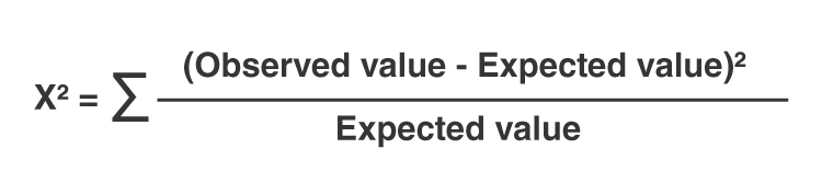
The Chi-Square Test is used to determine if there is a significant difference between the expected and observed data in categorical datasets. The formula for the Chi-Square statistic is:
$$ \chi^2 = \sum \frac{(O_i - E_i)^2}{E_i} $$
Where:
- \( \chi^2 \) is the Chi-Square statistic.
- \( O_i \) represents the observed frequency.
- \( E_i \) represents the expected frequency.
- \( \sum \) indicates the summation over all categories.
The steps to calculate the Chi-Square statistic are as follows:
- Calculate the expected frequencies for each category.
- Subtract the expected frequency from the observed frequency for each category.
- Square the result for each category.
- Divide the squared result by the expected frequency for each category.
- Sum all the values obtained in the previous step to get the Chi-Square statistic.
To better understand the formula, consider the following table which summarizes the steps:
| Category | Observed Frequency (O) | Expected Frequency (E) | (O - E) | (O - E)^2 | (O - E)^2 / E |
|---|---|---|---|---|---|
| A | OA | EA | OA - EA | (OA - EA)^2 | ((OA - EA)^2) / EA |
| B | OB | EB | OB - EB | (OB - EB)^2 | ((OB - EB)^2) / EB |
| ... | ... | ... | ... | ... | ... |
Once the Chi-Square statistic is calculated, it can be compared to a critical value from the Chi-Square distribution table with the appropriate degrees of freedom to determine the significance of the result.
Chi-Square Goodness-of-Fit Test
The Chi-Square Goodness-of-Fit Test is used to determine if a sample data matches a population with a specific distribution. This test is commonly used when you have one categorical variable from a single population and want to compare the observed frequencies of the categories to the expected frequencies, which are often based on a theoretical distribution.
Formula
The formula for the chi-square statistic is:
\[
\chi^2 = \sum \frac{(O_i - E_i)^2}{E_i}
\]
where:
- \(\chi^2\) = Chi-Square test statistic
- \(O_i\) = Observed frequency
- \(E_i\) = Expected frequency
- \(\sum\) = Summation over all categories
Steps to Perform a Chi-Square Goodness-of-Fit Test
- State the hypotheses:
- Null hypothesis (\(H_0\)): The observed frequencies match the expected frequencies.
- Alternative hypothesis (\(H_A\)): The observed frequencies do not match the expected frequencies.
- Calculate the expected frequencies:
Determine the expected frequency for each category based on the theoretical distribution. For example, if you expect equal distribution across categories, divide the total number of observations by the number of categories.
- Compute the chi-square statistic:
Use the formula to calculate the chi-square statistic.
\[
\chi^2 = \sum \frac{(O_i - E_i)^2}{E_i}
\] - Determine the degrees of freedom (df):
The degrees of freedom for the goodness-of-fit test is calculated as:
\[
\text{df} = \text{Number of categories} - 1
\] - Find the critical value and compare:
Use a chi-square distribution table to find the critical value at your desired significance level (e.g., \(\alpha = 0.05\)). Compare your computed chi-square statistic to this critical value.
- Make a decision:
- If the chi-square statistic is greater than the critical value, reject the null hypothesis.
- If the chi-square statistic is less than or equal to the critical value, do not reject the null hypothesis.
Example
Suppose a biologist claims that an equal number of four different species of deer enter a certain area each week. The observed frequencies over one week are:
- Species 1: 22
- Species 2: 20
- Species 3: 23
- Species 4: 35
The expected frequency for each species (assuming equal distribution) would be:
\[
E_i = \frac{22 + 20 + 23 + 35}{4} = 25
\]
Calculate the chi-square statistic:
\[
\chi^2 = \frac{(22 - 25)^2}{25} + \frac{(20 - 25)^2}{25} + \frac{(23 - 25)^2}{25} + \frac{(35 - 25)^2}{25} = 3.32
\]
With 3 degrees of freedom (4 categories - 1), and a significance level of 0.05, the critical value from the chi-square distribution table is approximately 7.815. Since 3.32 is less than 7.815, we do not reject the null hypothesis, indicating there is no significant difference between the observed and expected frequencies.
Chi-Square Test for Independence
The Chi-Square Test for Independence is used to determine if there is a significant association between two categorical variables. The test is based on the comparison of observed frequencies in each category to the frequencies we would expect if there was no association between the variables.
Steps to Perform the Chi-Square Test for Independence
-
State the Hypotheses:
- Null Hypothesis (\(H_0\)): The two variables are independent (no association).
- Alternative Hypothesis (\(H_a\)): The two variables are dependent (there is an association).
-
Construct the Contingency Table:
Arrange the data into a contingency table, where the rows represent the categories of one variable and the columns represent the categories of the other variable.
Category 1 Category 2 Total Group 1 \(O_{11}\) \(O_{12}\) \(Row 1 Total\) Group 2 \(O_{21}\) \(O_{22}\) \(Row 2 Total\) Total \(Col 1 Total\) \(Col 2 Total\) \(Grand Total\) -
Calculate the Expected Frequencies:
The expected frequency for each cell is calculated using the formula:
\[
E_{ij} = \frac{(\text{Row Total}) \times (\text{Column Total})}{\text{Grand Total}}
\] -
Compute the Chi-Square Test Statistic:
Use the observed (\(O_{ij}\)) and expected (\(E_{ij}\)) frequencies to calculate the chi-square statistic:
\[
\chi^2 = \sum \frac{(O_{ij} - E_{ij})^2}{E_{ij}}
\] -
Determine the Degrees of Freedom:
The degrees of freedom (df) for the test is calculated as:
\[
\text{df} = (r - 1) \times (c - 1)
\]where \(r\) is the number of rows and \(c\) is the number of columns.
-
Find the Critical Value and Compare:
Using the chi-square distribution table or a statistical software, find the critical value for the given degrees of freedom and the chosen significance level (\(\alpha\), typically 0.05). Compare the calculated chi-square statistic to the critical value.
-
Make a Decision:
- If \(\chi^2\) is greater than the critical value, reject the null hypothesis (\(H_0\)).
- If \(\chi^2\) is less than or equal to the critical value, do not reject the null hypothesis (\(H_0\)).
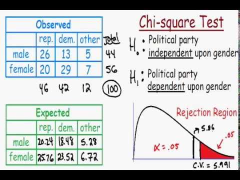
Example
Suppose a researcher wants to know whether gender is associated with political party preference. A random sample of 500 voters is surveyed, and the results are summarized in the following table:
| Republican | Democrat | Independent | Total | |
|---|---|---|---|---|
| Male | 120 | 90 | 40 | 250 |
| Female | 110 | 95 | 45 | 250 |
| Total | 230 | 185 | 85 | 500 |
Using the steps outlined above, the expected frequencies are calculated, the chi-square test statistic is computed, and the result is compared with the critical value to determine whether there is an association between gender and political party preference.
Example Problem 2: Test for Independence
In this example, we will perform a chi-square test for independence to determine if there is an association between gender and political party preference. The data from a survey of 440 voters is provided below:
| Republican | Democrat | Independent | Total | |
|---|---|---|---|---|
| Male | 100 | 70 | 30 | 200 |
| Female | 140 | 60 | 20 | 220 |
| Total | 240 | 130 | 50 | 440 |
Step-by-Step Solution
-
State the hypotheses:
- \( H_0 \): There is no association between gender and political party preference.
- \( H_a \): There is an association between gender and political party preference.
-
Calculate the expected frequencies:
Use the formula:
\[ \text{Expected Frequency} = \frac{(\text{Row Total} \times \text{Column Total})}{\text{Grand Total}} \]
For example, the expected frequency for Male Republicans is:
\[ \frac{(200 \times 240)}{440} = 109.09 \]
Similarly, calculate the expected frequencies for all cells:
Republican Democrat Independent Total Male 109.09 59.09 31.82 200 Female 130.91 70.91 38.18 220 Total 240 130 50 440 -
Compute the chi-square test statistic:
Use the formula:
\[ \chi^2 = \sum \frac{(O_i - E_i)^2}{E_i} \]
Where \( O_i \) is the observed frequency and \( E_i \) is the expected frequency. Compute this for each cell:
Republican Democrat Independent Male \[ \frac{(100 - 109.09)^2}{109.09} = 0.758 \] \[ \frac{(70 - 59.09)^2}{59.09} = 1.993 \] \[ \frac{(30 - 31.82)^2}{31.82} = 0.104 \] Female \[ \frac{(140 - 130.91)^2}{130.91} = 0.636 \] \[ \frac{(60 - 70.91)^2}{70.91} = 1.678 \] \[ \frac{(20 - 18.18)^2}{18.18} = 0.181 \] Summing these values gives:
\[ \chi^2 = 0.758 + 1.993 + 0.104 + 0.636 + 1.678 + 0.181 = 5.35 \]
-
Determine the degrees of freedom:
Degrees of freedom (df) are calculated as:
\[ \text{df} = (r - 1) \times (c - 1) \]
For this example:
\[ \text{df} = (2 - 1) \times (3 - 1) = 2 \]
-
Compare the chi-square statistic to the critical value:
Using a chi-square table or calculator with \( \alpha = 0.05 \) and \( \text{df} = 2 \), the critical value is 5.991.
Since our calculated \( \chi^2 \) value of 5.35 is less than the critical value of 5.991, we do not reject the null hypothesis.
-
Conclusion:
There is insufficient evidence to suggest an association between gender and political party preference.
Chi-Square Test for Homogeneity
The Chi-Square Test for Homogeneity is used to determine whether different populations have the same distribution of a single categorical variable. This test is similar to the Chi-Square Test for Independence, but it specifically compares the distribution of categories across different populations rather than assessing the association between two variables within a single population.
Steps to Perform a Chi-Square Test for Homogeneity
- State the Hypotheses
- Null Hypothesis (\( H_0 \)): The distributions of the categorical variable are the same across different populations.
- Alternative Hypothesis (\( H_a \)): The distributions of the categorical variable are different across different populations.
- Collect the Data
Gather data in a contingency table format where rows represent different populations and columns represent the categories of the variable.
- Calculate the Expected Frequencies
The expected frequency for each cell is calculated using the formula:
\[
E_{ij} = \frac{(R_i \times C_j)}{N}
\]- \( E_{ij} \): Expected frequency for the cell in the \(i\)-th row and \(j\)-th column
- \( R_i \): Total number of observations in the \(i\)-th row
- \( C_j \): Total number of observations in the \(j\)-th column
- \( N \): Total number of observations
- Compute the Chi-Square Statistic
The Chi-Square statistic is calculated using the formula:
\[
\chi^2 = \sum \frac{(O_{ij} - E_{ij})^2}{E_{ij}}
\]- \( O_{ij} \): Observed frequency for the cell in the \(i\)-th row and \(j\)-th column
- \( E_{ij} \): Expected frequency for the cell in the \(i\)-th row and \(j\)-th column
- Determine the Degrees of Freedom
The degrees of freedom (df) for the test is calculated as:
\[
df = (r - 1) \times (c - 1)
\]- \( r \): Number of rows
- \( c \): Number of columns
- Find the Critical Value and Make a Decision
Compare the calculated Chi-Square statistic to the critical value from the Chi-Square distribution table at the desired significance level (usually 0.05). If the Chi-Square statistic is greater than the critical value, reject the null hypothesis.
Example Problem: Test for Homogeneity
Suppose a researcher wants to determine if three different teaching methods lead to different pass rates among students. The results are as follows:
| Teaching Method | Pass | Fail |
|---|---|---|
| Method A | 30 | 10 |
| Method B | 25 | 15 |
| Method C | 20 | 20 |
Step-by-Step Solution:
- State the hypotheses:
- \( H_0 \): The pass rates are the same for all teaching methods.
- \( H_a \): The pass rates are different for at least one teaching method.
- Calculate the expected frequencies for each cell:
\[
E_{ij} = \frac{(R_i \times C_j)}{N}
\]- For Method A (Pass): \( E_{11} = \frac{40 \times 75}{120} = 25 \)
- For Method A (Fail): \( E_{12} = \frac{40 \times 45}{120} = 15 \)
- Continue this process for all cells.
- Compute the Chi-Square statistic:
\[
\chi^2 = \sum \frac{(O_{ij} - E_{ij})^2}{E_{ij}}
\]- \( \chi^2 = \frac{(30 - 25)^2}{25} + \frac{(10 - 15)^2}{15} + \ldots \)
- Calculate the sum for all cells.
- Determine the degrees of freedom:
\[
df = (3 - 1) \times (2 - 1) = 2
\] - Compare the Chi-Square statistic to the critical value and make a decision.
- If the calculated \( \chi^2 \) is greater than the critical value at \( df = 2 \) and \( \alpha = 0.05 \), reject \( H_0 \).
Example Problem 3: Test for Homogeneity
Suppose we want to determine if the distribution of preferred pet types (cats, dogs, and birds) varies across different age groups. We survey 300 individuals categorized into three age groups: 18-30 years, 31-50 years, and over 50 years.
Here are the observed frequencies:
| Cats | Dogs | Birds | |
| 18-30 years | 50 | 100 | 30 |
| 31-50 years | 30 | 60 | 10 |
| Over 50 years | 20 | 40 | 10 |
First, we state the null hypothesis, \( H_0 \): The distribution of preferred pet types is the same across all age groups.
To perform the chi-square test for homogeneity, calculate the expected frequencies under the assumption of homogeneity:
- Calculate row totals and column totals.
- Compute the overall total, \( n = 300 \).
- Calculate the expected frequency for each cell using the formula: \[ E_{ij} = \frac{(\text{row total}_i \times \text{column total}_j)}{n} \]
- Perform the chi-square test statistic calculation: \[ \chi^2 = \sum \frac{(O_{ij} - E_{ij})^2}{E_{ij}} \]
- Determine the degrees of freedom, \( df = (r - 1)(c - 1) \), where \( r \) is the number of rows and \( c \) is the number of columns.
- Compare the calculated chi-square statistic to the critical value from the chi-square distribution table at a chosen significance level (e.g., 0.05).
If \( \chi^2 \) is greater than the critical value, reject the null hypothesis and conclude that there is evidence that the distribution of preferred pet types varies across age groups. Otherwise, fail to reject the null hypothesis.
Interpret the results and make conclusions based on the findings of the test.
Interpreting Chi-Square Test Results
After performing a chi-square test, you obtain a chi-square statistic and its associated p-value. Here’s how to interpret the results:
- Compare the chi-square statistic to the critical value:
- If \( \chi^2 \) is greater than the critical value from the chi-square distribution table at a chosen significance level (e.g., 0.05), this suggests that there is evidence of a significant relationship between the variables.
- If \( \chi^2 \) is less than the critical value, there is insufficient evidence to reject the null hypothesis, indicating no significant relationship between the variables.
- Examine the p-value:
- If the p-value is less than the chosen significance level (e.g., 0.05), reject the null hypothesis. This indicates that the observed frequencies differ significantly from the expected frequencies, suggesting a significant relationship between the variables.
- If the p-value is greater than the significance level, do not reject the null hypothesis. This suggests that the observed frequencies do not differ significantly from the expected frequencies, indicating no significant relationship between the variables.
- Consider the degrees of freedom:
- Degrees of freedom (\( df \)) are calculated as \( (r-1)(c-1) \), where \( r \) is the number of rows and \( c \) is the number of columns in the contingency table.
- A higher degrees of freedom value indicates more variability and flexibility in interpreting the chi-square statistic.
- Conclusion:
- Based on the results of the chi-square test, make a conclusion about the relationship between the variables. Clearly state whether you reject or fail to reject the null hypothesis and interpret the practical significance of the findings.
Common Mistakes in Chi-Square Tests
When performing chi-square tests, avoid these common mistakes to ensure accurate results:
- Small Sample Sizes: Using chi-square tests with small sample sizes can lead to unreliable results, as the test may not have enough power to detect true associations.
- Incorrect Application: Misapplying chi-square tests by using them for continuous data or data that violates the test assumptions (e.g., expected cell counts less than 5) can yield inaccurate conclusions.
- Violating Independence Assumption: Failing to ensure that observations are independent can invalidate the results of the chi-square test, as it assumes each observation is independent of the others.
- Improper Interpretation of Results: Misinterpreting the chi-square statistic or p-value without considering the context of the study or the assumptions of the test can lead to erroneous conclusions.
- Not Checking Assumptions: Neglecting to verify if the assumptions of the chi-square test (e.g., expected frequencies, random sampling) are met can undermine the validity of the results.
- Confusing Chi-Square Tests: Mixing up different types of chi-square tests (e.g., goodness-of-fit, test for independence, test for homogeneity) and applying them incorrectly to the data can lead to incorrect conclusions.
By avoiding these common pitfalls and ensuring proper application of the chi-square test, researchers can obtain reliable and meaningful results that accurately reflect the relationships within their data.
Chi-Square Test FAQs
- What is a chi-square test?
A chi-square test is a statistical method used to determine if there is a significant association between categorical variables.
- When should I use a chi-square test?
Use a chi-square test when you have categorical data and want to determine if there is a relationship or association between two or more variables.
- What are the types of chi-square tests?
The main types of chi-square tests include:
- Goodness-of-Fit Test: Compares observed frequencies to expected frequencies.
- Test for Independence: Determines if there is a relationship between two categorical variables.
- Test for Homogeneity: Assesses whether the distribution of a categorical variable is similar across different groups.
- What are the assumptions of the chi-square test?
The assumptions include:
- Each observation must be independent.
- Expected frequencies should be greater than 5 for most cells.
- The variables being studied must be categorical.
- How do you interpret the results of a chi-square test?
Interpret the results by comparing the calculated chi-square statistic to the critical value from the chi-square distribution table at a chosen significance level (e.g., 0.05). Additionally, examine the p-value: a low p-value indicates a significant relationship between the variables.
- What should I do if the assumptions of the chi-square test are violated?
If assumptions are violated (e.g., expected frequencies are less than 5), consider using alternative tests or adjusting the data to meet the assumptions.
- Can chi-square test be used for continuous data?
No, chi-square tests are specifically designed for categorical data. For continuous data, other tests such as t-tests or ANOVA should be used.
Conclusion
In conclusion, the chi-square test is a powerful tool for analyzing categorical data and determining relationships between variables. By following the steps outlined in this guide, researchers can:
- Understand the basics of the chi-square test, including its purpose and types.
- Learn how to perform and interpret a chi-square test correctly.
- Avoid common mistakes that can affect the validity of chi-square test results.
- Use chi-square tests to make informed decisions based on statistical evidence.
Whether conducting research in social sciences, biology, business, or any other field that involves categorical data, mastering the chi-square test allows for deeper insights into relationships and distributions. By applying this statistical method effectively, researchers contribute to the advancement of knowledge and evidence-based decision-making.
Xem bài giảng về kiểm định Goodness of Fit sử dụng phương pháp Kiểm Định Chi Square trong Toán Kỹ Thuật 4.
Kiểm Định Goodness of Fit - Bài 1 - Kiểm Định Chi Square - Toán Kỹ Thuật 4
READ MORE:
Kiểm Định Chi-Square || Sự Phù Hợp || Toàn Bộ Khái Niệm Kiểm Định Chi-Square Trong 1 Video bởi Arya Anjum


:max_bytes(150000):strip_icc()/Chi-SquareStatistic_Final_4199464-7eebcd71a4bf4d9ca1a88d278845e674.jpg)