Topic chi-square test genetics example: The chi-square test is essential in genetics for analyzing and interpreting data. This article explores chi-square test applications in genetics, providing detailed examples and step-by-step guidance to help you understand and apply this statistical tool effectively. Whether you're a student or researcher, mastering chi-square tests can significantly enhance your genetic data analysis skills.
Table of Content
- Chi-Square Test in Genetics
- Introduction
- Overview of Chi-Square Test
- When to Use Chi-Square Test
- Chi-Square Test Formula
- Steps to Perform a Chi-Square Test
- Examples of Chi-Square Tests in Genetics
- Chi-Square Test for Goodness of Fit
- Chi-Square Test for Independence
- Using Chi-Square Tests in Plant Breeding
- YOUTUBE: Video về Phân tích Chi Square và Các Sự giao thoa di truyền giúp bạn hiểu sâu hơn về cách áp dụng kiểm định này trong các ví dụ thực tế về di truyền.
Chi-Square Test in Genetics
The chi-square test is a statistical method used to determine if there is a significant difference between the expected and observed frequencies in categorical data. This test is commonly used in genetics to analyze the results of genetic crosses and to test the fit of observed data to expected Mendelian ratios.
Null Hypothesis
The null hypothesis for a chi-square test in genetics typically states that there is no significant difference between the observed and expected frequencies. This implies that any deviations from expected values are due to random chance.
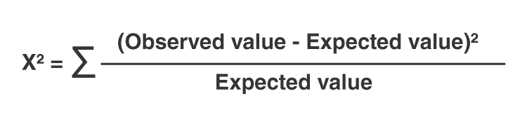
Chi-Square Formula
The formula for the chi-square test is:
$$
\chi^2 = \sum \frac{(O_i - E_i)^2}{E_i}
$$
where \( O_i \) is the observed frequency and \( E_i \) is the expected frequency for each category.
Example Calculation
Let's consider an example where we test the fit of observed data to a 9:3:3:1 ratio in a dihybrid cross:
| Phenotype | Observed (O) | Expected (E) | \(O - E\) | \((O - E)^2\) | \(\frac{(O - E)^2}{E}\) |
|---|---|---|---|---|---|
| Round, Yellow | 315 | 312.75 | 2.25 | 5.0625 | 0.0162 |
| Round, Green | 108 | 104.25 | 3.75 | 14.0625 | 0.1349 |
| Wrinkled, Yellow | 101 | 104.25 | -3.25 | 10.5625 | 0.1013 |
| Wrinkled, Green | 32 | 34.75 | -2.75 | 7.5625 | 0.2176 |
The sum of the last column gives the chi-square value:
$$
\chi^2 = 0.0162 + 0.1349 + 0.1013 + 0.2176 = 0.47
$$
Degrees of Freedom
The degrees of freedom (df) for this test is calculated as the number of categories minus one:
$$
df = n - 1 = 4 - 1 = 3
$$
Interpreting the Result
Using a chi-square table, we compare the calculated chi-square value with the critical value at \( df = 3 \) and a significance level (typically 0.05). If the chi-square value is less than the critical value, we accept the null hypothesis, indicating that any observed differences are due to chance. In this example, with a chi-square value of 0.47 and df of 3, the result is not significant at the 0.05 level, so we accept the null hypothesis.
Conclusion
The chi-square test is a vital tool in genetics for validating the fit of observed data to expected genetic ratios. It helps in confirming hypotheses about genetic inheritance patterns and detecting significant deviations that might indicate other underlying factors.

READ MORE:
Introduction
The chi-square test is a statistical method used to determine if there is a significant difference between observed and expected frequencies in categorical data. This test is particularly useful in genetics for evaluating whether experimental data fits a theoretical distribution, such as Mendelian inheritance ratios. The chi-square test can assess both the goodness of fit and the independence between different genetic traits.
In a typical genetics example, the chi-square test helps in testing hypotheses about the distribution of phenotypes. For instance, Mendel's experiments with pea plants predicted a 3:1 ratio of dominant to recessive traits. The chi-square test is used to determine whether the observed data from such an experiment significantly deviates from the expected ratio.
Here are the main steps involved in performing a chi-square test in genetics:
- State the null hypothesis, which assumes no significant difference between observed and expected values.
- Collect and categorize the observed data.
- Calculate the expected frequencies based on the theoretical model.
- Use the chi-square formula to compute the test statistic:
\[
X^2 = \sum \frac{(O - E)^2}{E}
\]
where \(X^2\) is the chi-square statistic, \(O\) is the observed frequency, and \(E\) is the expected frequency. - Determine the degrees of freedom, which is the number of categories minus one.
- Compare the calculated chi-square value to the critical value from the chi-square distribution table to determine the p-value.
- Accept or reject the null hypothesis based on the p-value and a predetermined significance level (e.g., 0.05).
Overview of Chi-Square Test
The Chi-Square test is a statistical method used to determine if there is a significant difference between the observed and expected frequencies in categorical data. It is widely used in genetics to test hypotheses about the distribution of traits in a population, following Mendelian inheritance patterns.
- Purpose: To assess if the observed frequencies of events differ from the expected frequencies based on a specific hypothesis.
- Types:
- Chi-Square Goodness of Fit Test: Tests if sample data matches a population with a specific distribution.
- Chi-Square Test of Independence: Tests if two categorical variables are independent of each other.
Steps to Perform a Chi-Square Test
- Formulate Hypotheses:
- Null Hypothesis (H0): Assumes no significant difference between the observed and expected frequencies.
- Alternative Hypothesis (H1): Assumes a significant difference between the observed and expected frequencies.
- Calculate Expected Frequencies: Based on the theoretical distribution or genetic ratio (e.g., 9:3:3:1 ratio in dihybrid crosses).
- Compute Chi-Square Statistic: Using the formula:
$$\chi^2 = \sum \frac{(O_i - E_i)^2}{E_i}$$
where \( O_i \) is the observed frequency and \( E_i \) is the expected frequency. - Determine Degrees of Freedom (df): Calculated as \( \text{df} = \text{number of categories} - 1 \).
- Compare with Critical Value: Use a Chi-Square distribution table to find the critical value for the given degrees of freedom and significance level (usually 0.05).
- If \( \chi^2 \) value is greater than the critical value, reject the null hypothesis.
- If \( \chi^2 \) value is less than the critical value, fail to reject the null hypothesis.
The Chi-Square test is a versatile tool in genetics for validating theoretical ratios and understanding the distribution of genetic traits. It helps researchers confirm or refute the expected inheritance patterns and explore the potential factors affecting genetic variation.
| Category | Observed (O) | Expected (E) | (O - E) | (O - E)2 | \(\frac{(O - E)^2}{E}\) |
|---|---|---|---|---|---|
| Category 1 | 50 | 45 | 5 | 25 | 0.56 |
| Category 2 | 30 | 35 | -5 | 25 | 0.71 |
| Category 3 | 20 | 20 | 0 | 0 | 0 |
| Total | 100 | 100 | 1.27 |
When to Use Chi-Square Test
The Chi-Square test is a statistical method used to determine if there is a significant association between categorical variables. In genetics, it is particularly useful for analyzing the distribution of different phenotypes and determining whether observed genetic data fits expected Mendelian ratios. Here are some scenarios where you might use a Chi-Square test in genetics:
- Goodness of Fit: When you want to test if the observed distribution of phenotypes matches the expected distribution based on Mendelian inheritance. For example, testing if the ratio of offspring phenotypes in a genetic cross fits the expected 9:3:3:1 ratio.
- Test of Independence: When you want to determine if there is a significant association between two categorical variables. For instance, checking if the occurrence of a specific genetic trait is independent of another trait or factor, such as gender or environmental exposure.
- Homogeneity: When comparing the distributions of a categorical variable across different populations to see if they are the same. For example, comparing the frequency of a genetic trait in different geographical populations.
The test involves calculating the Chi-Square statistic from observed and expected frequencies, and comparing it to a critical value from the Chi-Square distribution table. If the calculated value exceeds the critical value, it suggests that the observed deviations are not due to chance, indicating a significant difference or association.
Chi-Square Test Formula
The chi-square test is a statistical method used to determine if there is a significant difference between the expected and observed frequencies in one or more categories. The formula for the chi-square test is:
$$
\chi^2 = \sum \frac{(O - E)^2}{E}
$$
where:
- \(\chi^2\) is the chi-square statistic
- O represents the observed frequency
- E represents the expected frequency
The steps to calculate the chi-square statistic are as follows:
- Calculate the expected frequencies based on the null hypothesis.
- Compute the differences between the observed and expected frequencies.
- Square each difference.
- Divide each squared difference by the expected frequency.
- Sum all the values obtained in the previous step to get the chi-square statistic.
The degrees of freedom for the chi-square test are calculated as:
$$
\text{df} = n - 1
$$
where \( n \) is the number of categories.
To interpret the chi-square statistic, compare it against a critical value from the chi-square distribution table. If the calculated chi-square value exceeds the critical value at a given significance level (e.g., 0.05), the null hypothesis is rejected, indicating a significant difference between the observed and expected frequencies.
Steps to Perform a Chi-Square Test
Performing a Chi-Square test involves several methodical steps to ensure accurate results. Here's a detailed, step-by-step guide:
-
Define the Hypothesis:
Start by defining the null hypothesis (H0) and the alternative hypothesis (Ha). The null hypothesis typically states that there is no significant difference between the observed and expected frequencies.
-
Collect Data:
Gather your observed data. This data should be categorized into distinct groups or categories relevant to your study.
-
Calculate Expected Frequencies:
For each category, calculate the expected frequencies. This is done using the formula:
Expected Frequency (E) = (Row Total * Column Total) / Grand Total -
Compute the Chi-Square Statistic:
Use the Chi-Square formula to calculate the test statistic:
\[
\chi^2 = \sum \frac{(O - E)^2}{E}
\]- O = Observed frequency
- E = Expected frequency
-
Determine Degrees of Freedom:
The degrees of freedom (df) is calculated using the formula:
\[
df = (r - 1) \times (c - 1)
\]- r = number of rows
- c = number of columns
-
Find the Critical Value:
Using a Chi-Square distribution table, find the critical value corresponding to your calculated degrees of freedom and the desired significance level (commonly 0.05).
-
Compare and Interpret:
Compare your Chi-Square statistic to the critical value. If the statistic exceeds the critical value, reject the null hypothesis. Otherwise, do not reject the null hypothesis.
Following these steps ensures a comprehensive approach to performing a Chi-Square test, providing a solid foundation for interpreting your genetic data accurately.
Examples of Chi-Square Tests in Genetics
The chi-square test is a crucial tool in genetics, allowing researchers to test hypotheses about genetic ratios. Here are some detailed examples of how this test is used in genetic studies:
-
Example 1: Mendelian Inheritance
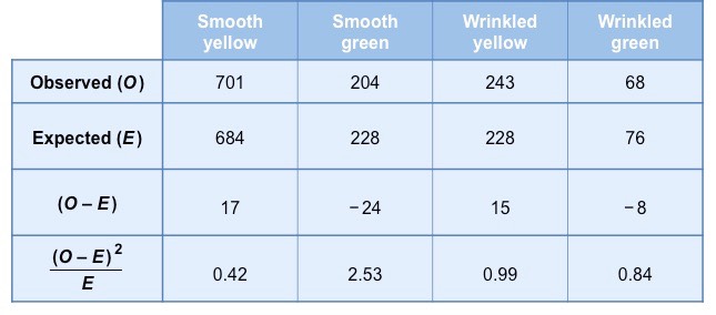
Consider a classic Mendelian dihybrid cross involving two traits: seed shape and seed color in pea plants. The expected phenotypic ratio for the F2 generation is 9:3:3:1. Suppose the observed counts are as follows:
Phenotype Observed Expected Round, Yellow 315 312.75 Round, Green 108 104.25 Wrinkled, Yellow 101 104.25 Wrinkled, Green 32 34.75 The chi-square value is calculated as:
\[ \chi^2 = \sum \frac{(O_i - E_i)^2}{E_i} \]Using this formula, the chi-square value for this data is 0.47. With 3 degrees of freedom, the p-value is greater than 0.90, indicating no significant deviation from the expected ratio.
-
Example 2: Monohybrid Cross
In a monohybrid cross of tall and short plants, the F2 generation yields 33 tall and 7 short plants. The expected ratio is 3:1. Here is the calculation:
Phenotype Observed Expected Tall 33 30 Short 7 10 Using the chi-square formula, the value is 1.2. With 1 degree of freedom, the p-value indicates that the null hypothesis cannot be rejected, supporting the expected 3:1 ratio.
-
Example 3: Plant Breeding
In a study of tomato plant disease resistance, a hypothesis of single gene inheritance is tested. The observed and expected counts of resistant and susceptible plants are compared using chi-square analysis to validate the inheritance pattern.
These examples illustrate the application of chi-square tests in genetics to determine if observed data fits expected Mendelian ratios, thereby validating genetic hypotheses.
Chi-Square Test for Goodness of Fit
The chi-square test for goodness of fit is a statistical test used to determine how well categorical data fits an expected distribution or hypothesis. In genetics, this test is particularly useful for examining whether observed genotype frequencies match expected frequencies based on Mendelian ratios or other genetic models.
Here’s a step-by-step outline of how to conduct a chi-square goodness of fit test:
- Formulate Hypotheses: Define the null hypothesis (H0) and alternative hypothesis (H1). For example, in Mendelian genetics, H0 might state that observed genotype frequencies fit the expected ratios (e.g., 1:2:1 for a monohybrid cross).
- Collect Data: Gather observed frequencies of each genotype from your experimental data.
- Calculate Expected Frequencies: Determine the expected frequencies for each genotype under the null hypothesis. This is often based on theoretical predictions (e.g., Mendelian ratios).
- Compute the Chi-Square Statistic: Use the formula:
\(\chi^2 = \sum \frac{{(O_i - E_i)^2}}{{E_i}}\)
where \( O_i \) is the observed frequency and \( E_i \) is the expected frequency for each genotype category.
- Determine Degrees of Freedom: Calculate degrees of freedom, typically \( df = n - 1 \), where \( n \) is the number of genotype categories minus 1.
- Find Critical Value: Look up the critical chi-square value for your chosen significance level and degrees of freedom in a chi-square table.
- Compare \(\chi^2\) Value: Compare your calculated \(\chi^2\) value with the critical value. If \(\chi^2\) is greater than the critical value, reject the null hypothesis.
- Interpret Results: Based on the comparison, decide whether the observed frequencies fit the expected distribution. This informs whether the genetic data supports or contradicts the null hypothesis.
This test is essential in genetics for validating genetic hypotheses and understanding deviations from expected outcomes, thereby contributing significantly to genetic research and breeding programs.
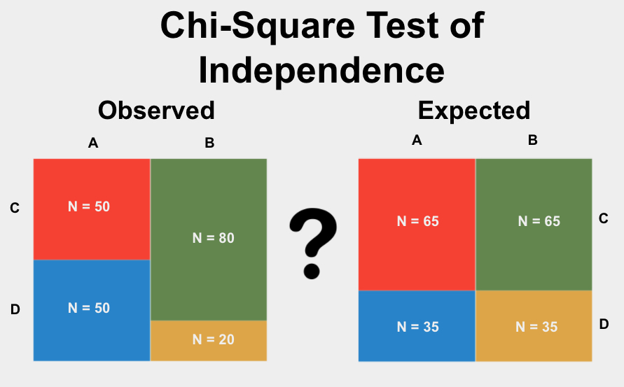
Chi-Square Test for Independence
The chi-square test for independence is a statistical test used to examine the relationship between two categorical variables. In genetics, this test is crucial for determining whether there is a significant association between different traits or genes.
Here’s a detailed outline of how to perform a chi-square test for independence:
- Formulate Hypotheses: Define the null hypothesis (H0) stating that there is no association between the variables, and the alternative hypothesis (H1) stating that there is an association.
- Collect Data: Gather observed frequencies for each combination of the two categorical variables from your genetic study.
- Create a Contingency Table: Construct a contingency table (also known as a cross-tabulation or two-way table) to organize the data.
- Calculate Expected Frequencies: Compute the expected frequencies for each cell in the contingency table under the assumption of independence.
- Compute the Chi-Square Statistic: Use the formula:
\(\chi^2 = \sum \frac{{(O_i - E_i)^2}}{{E_i}}\)
where \( O_i \) is the observed frequency and \( E_i \) is the expected frequency for each cell in the contingency table.
- Determine Degrees of Freedom: Calculate degrees of freedom, typically \( df = (r - 1) \times (c - 1) \), where \( r \) is the number of rows and \( c \) is the number of columns in the contingency table.
- Find Critical Value: Look up the critical chi-square value for your chosen significance level and degrees of freedom in a chi-square table.
- Compare \(\chi^2\) Value: Compare your calculated \(\chi^2\) value with the critical value. If \(\chi^2\) is greater than the critical value, reject the null hypothesis.
- Interpret Results: Based on the comparison, determine whether there is a statistically significant association between the variables. This helps geneticists understand how different traits or genes might be linked or inherited together.
The chi-square test for independence plays a crucial role in genetic studies by providing insights into genetic associations and dependencies, thereby advancing our understanding of inheritance patterns and genetic diversity.

Using Chi-Square Tests in Plant Breeding
Chi-square tests are invaluable in plant breeding for analyzing and interpreting data related to genetic traits and cross-breeding experiments. They provide statistical rigor to assess whether observed results conform to expected genetic ratios, helping breeders make informed decisions.
Here’s how chi-square tests are applied in plant breeding:
- Genetic Trait Analysis: Breeders use chi-square tests to determine whether observed phenotypic ratios in offspring match expected ratios based on genetic models.
- Cross-Breeding Experiments: Chi-square tests evaluate the independence of traits across different genetic crosses, revealing patterns of inheritance and potential genetic linkages.
- Selection Decisions: Breeders rely on chi-square tests to validate breeding goals and select plants that exhibit desired genetic traits with statistical confidence.
- Population Genetics: Chi-square tests aid in studying genetic diversity within populations, identifying allele frequencies, and assessing deviations from Hardy-Weinberg equilibrium.
- Quantitative Trait Loci (QTL) Mapping: Chi-square tests help in mapping QTLs by analyzing associations between molecular markers and trait variations.
By employing chi-square tests, plant breeders enhance breeding efficiency, ensure genetic purity, and accelerate the development of new cultivars with improved traits. This statistical approach contributes significantly to advancing agricultural productivity and sustainability.
Video về Phân tích Chi Square và Các Sự giao thoa di truyền giúp bạn hiểu sâu hơn về cách áp dụng kiểm định này trong các ví dụ thực tế về di truyền.
Phân tích Chi Square và Các Sự giao thoa di truyền
READ MORE:
Video về Kiểm định Chi Square và Các Bài toán Di truyền sẽ giúp bạn giải quyết các vấn đề liên quan đến di truyền một cách hiệu quả, áp dụng kiến thức vào thực tế.
Kiểm định Chi Square và Các Bài toán Di truyền


:max_bytes(150000):strip_icc()/Chi-SquareStatistic_Final_4199464-7eebcd71a4bf4d9ca1a88d278845e674.jpg)