Topic z-test vs chi-square: When it comes to statistical analysis, choosing the right test is crucial. In this article, we'll explore the differences between the Z-Test and the Chi-Square test, both essential tools for hypothesis testing. Learn how each test works, their applications, and when to use them for your data analysis needs.
Table of Content
- Z-Test vs Chi-Square Test
- Introduction to Z-Test and Chi-Square Test
- Z-Test Formula and Calculation
- Examples of Z-Test Applications
- Chi-Square Test Types
- Chi-Square Goodness of Fit Test
- Chi-Square Test of Independence
- Chi-Square Formula and Calculation
- Examples of Chi-Square Applications
- Comparison Between Z-Test and Chi-Square Test
- Key Differences
- Advantages and Disadvantages
- Common Mistakes and How to Avoid Them
- Conclusion
- YOUTUBE: Video giải thích về kiểm định Chi-Square. Hướng dẫn chi tiết và dễ hiểu về phương pháp kiểm định quan trọng này trong thống kê.
Z-Test vs Chi-Square Test
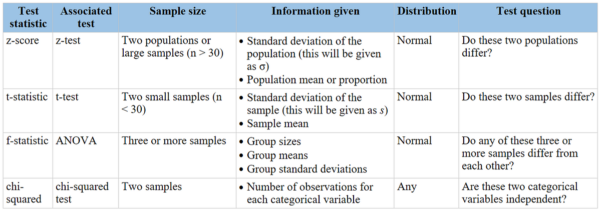
In statistics, both Z-tests and Chi-square tests are used to determine if there is a significant difference between observed data and what is expected under the null hypothesis. However, they serve different purposes and are used in different scenarios.
Z-Test
The Z-test is used when the data follows a normal distribution and the sample size is large (typically n > 30). It is primarily used to compare sample and population means to see if there is a significant difference.
When to Use a Z-Test
- Large sample sizes (n > 30)
- Known population variance
- Comparing sample means to a population mean
Z-Test Formula
For a sample mean, the Z-test formula is:
$$ Z = \frac{\bar{X} - \mu}{\frac{\sigma}{\sqrt{n}}} $$
where:
- \(\bar{X}\) = sample mean
- \(\mu\) = population mean
- \(\sigma\) = population standard deviation
- n = sample size
Chi-Square Test
The Chi-square test is used to determine if there is a significant association between categorical variables. It is a non-parametric test, meaning it does not assume a normal distribution of the data.
Types of Chi-Square Tests
- Chi-Square Goodness of Fit Test: Determines if a sample matches the expected distribution.
- Chi-Square Test of Independence: Assesses if two categorical variables are independent.
Chi-Square Test Formula
The formula for the Chi-square test is:
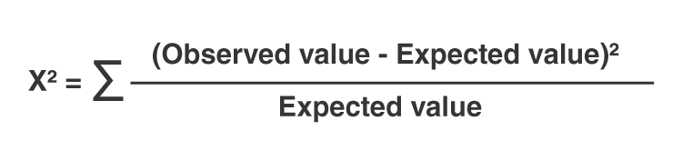
$$ \chi^2 = \sum \frac{(O_i - E_i)^2}{E_i} $$
where:
- \(O_i\) = observed frequency
- \(E_i\) = expected frequency
When to Use a Chi-Square Test
- Categorical data
- Testing for independence between variables
- Testing goodness of fit
Comparison of Z-Test and Chi-Square Test
| Aspect | Z-Test | Chi-Square Test |
|---|---|---|
| Data Type | Continuous | Categorical |
| Sample Size | Large (n > 30) | Varies (usually larger for accurate results) |
| Distribution | Normal | Non-parametric |
| Purpose | Comparing sample mean to population mean | Testing independence or goodness of fit |
In summary, the choice between a Z-test and a Chi-square test depends on the type of data you have and the hypothesis you are testing. Understanding the differences and appropriate applications of each test ensures accurate and meaningful statistical analysis.

READ MORE:
Introduction to Z-Test and Chi-Square Test
The Z-Test and Chi-Square Test are essential tools in statistics for hypothesis testing and data analysis. Both tests serve different purposes and are used under specific conditions. Understanding the differences between them helps in selecting the appropriate test for your data analysis.
The Z-Test is used when comparing a sample mean to a known population mean, especially when the sample size is large (n > 30) and the population standard deviation is known. It assumes that the data follows a normal distribution. The test statistic for the Z-Test is calculated as:
\[
Z = \frac{\bar{X} - \mu}{\sigma / \sqrt{n}}
\]
where:
- \(\bar{X}\) is the sample mean
- \(\mu\) is the population mean
- \(\sigma\) is the population standard deviation
- n is the sample size
The Z-Test helps determine if there is a significant difference between the sample mean and the population mean.
The Chi-Square Test is used for testing relationships between categorical variables. It evaluates whether the observed frequencies in each category match the expected frequencies. The Chi-Square statistic is calculated as:
\[
\chi^2 = \sum \frac{(O_i - E_i)^2}{E_i}
\]
where:
- \(O_i\) is the observed frequency
- \(E_i\) is the expected frequency
The Chi-Square Test is particularly useful in assessing the goodness of fit and testing for independence in contingency tables. It requires that the expected frequency in each category is at least 5 to ensure validity.
In summary, the Z-Test is optimal for continuous data and comparing means, while the Chi-Square Test is ideal for categorical data and testing associations. Choosing the correct test depends on the data type and the specific hypothesis being tested.
Z-Test Formula and Calculation
The Z-test is a statistical method used to determine if there is a significant difference between the means of two datasets. It is typically used when the population variance is known and the sample size is large (n > 30). Below, we detail the formula and steps for calculating the Z-test statistic.
One-Sample Z-Test Formula
The one-sample Z-test formula is used to compare the mean of a single sample to a known population mean. The formula is given by:
$$
Z = \frac{\overline{x} - \mu}{\frac{\sigma}{\sqrt{n}}}
$$
- \(\overline{x}\): Sample mean
- \(\mu\): Population mean
- \(\sigma\): Population standard deviation
- n: Sample size
Two-Sample Z-Test Formula
The two-sample Z-test formula is used to compare the means of two independent samples. The formula is given by:
$$
Z = \frac{(\overline{x_1} - \overline{x_2}) - (\mu_1 - \mu_2)}{\sqrt{\frac{\sigma_1^2}{n_1} + \frac{\sigma_2^2}{n_2}}}
$$
- \(\overline{x_1}\), \(\overline{x_2}\): Sample means of the two groups
- \(\mu_1\), \(\mu_2\): Population means of the two groups (often assumed to be equal under the null hypothesis)
- \(\sigma_1\), \(\sigma_2\): Population standard deviations of the two groups
- n_1\), \(n_2\): Sample sizes of the two groups
Steps for Calculating the Z-Test
- State the hypotheses: Define the null hypothesis (\(H_0\)) and the alternative hypothesis (\(H_A\)).
- Choose the significance level (α): Common choices are 0.05, 0.01, and 0.10.
- Calculate the Z-test statistic: Use the appropriate formula depending on whether you are performing a one-sample or two-sample Z-test.
- Find the critical value: Using the Z-table, find the critical value that corresponds to the chosen significance level.
- Compare the test statistic to the critical value: If the test statistic exceeds the critical value (in absolute terms for a two-tailed test), reject the null hypothesis.
Example Calculation
Suppose a sample of 50 students has a mean test score of 85, while the population mean test score is 80 with a standard deviation of 10. To determine if this sample mean is significantly different from the population mean at the 0.05 significance level, we perform the following steps:
- Calculate the test statistic: $$ Z = \frac{85 - 80}{\frac{10}{\sqrt{50}}} = \frac{5}{1.41} \approx 3.54 $$
- Find the critical value for α = 0.05 (two-tailed test): ±1.96
- Compare the test statistic to the critical value: 3.54 > 1.96
Since 3.54 exceeds 1.96, we reject the null hypothesis, indicating that the sample mean is significantly different from the population mean.
Examples of Z-Test Applications
Z-tests are widely used in various fields for hypothesis testing. Below are detailed examples of applications of Z-tests to illustrate their utility:
-
Example 1: Education
A teacher claims that the mean score of students in his class is greater than 82 with a standard deviation of 20. A sample of 81 students has a mean score of 90. To test this claim at a 0.05 significance level, the following steps are performed:
- State the null hypothesis: \(H_0: \mu = 82\)
- State the alternative hypothesis: \(H_1: \mu > 82\)
- Calculate the Z-test statistic: \(z = \frac{\overline{x} - \mu}{\frac{\sigma}{\sqrt{n}}}\)
- Substitute the values: \(z = \frac{90 - 82}{\frac{20}{\sqrt{81}}} = 3.6\)
- Compare with the critical value: 3.6 > 1.645, thus reject the null hypothesis
Conclusion: There is enough evidence to support the teacher's claim.
-
Example 2: Healthcare
An online medicine shop claims that the mean delivery time for medicines is less than 120 minutes with a standard deviation of 30 minutes. A sample of 49 orders has a mean delivery time of 100 minutes. To test this claim at a 0.05 significance level, the following steps are performed:
- State the null hypothesis: \(H_0: \mu = 120\)
- State the alternative hypothesis: \(H_1: \mu < 120\)
- Calculate the Z-test statistic: \(z = \frac{\overline{x} - \mu}{\frac{\sigma}{\sqrt{n}}}\)
- Substitute the values: \(z = \frac{100 - 120}{\frac{30}{\sqrt{49}}} = -4.66\)
- Compare with the critical value: -4.66 < -1.645, thus reject the null hypothesis
Conclusion: There is enough evidence to support the medicine shop's claim.
-
Example 3: Manufacturing
A company wants to improve the quality of products by reducing defects and monitoring the efficiency of assembly lines. In assembly line A, there were 18 defects reported out of 200 samples while in line B, 25 defects out of 600 samples were noted. To test if there is a difference in the proportion of defects between the two lines, the following steps are performed:
- State the null hypothesis: \(H_0: p_1 = p_2\)
- State the alternative hypothesis: \(H_1: p_1 \neq p_2\)
- Calculate the pooled proportion: \(p = \frac{x_1 + x_2}{n_1 + n_2}\)
- Calculate the Z-test statistic: \(z = \frac{p_1 - p_2}{\sqrt{p(1-p)(\frac{1}{n_1} + \frac{1}{n_2})}}\)
- Substitute the values and compute the test statistic
- Compare with the critical value and make a decision
Conclusion: Based on the calculated Z-test statistic, determine if there is a significant difference in the defect rates.
Chi-Square Test Types
The chi-square test is a statistical method used to determine if there is a significant association between categorical variables. It is widely used in hypothesis testing to analyze the relationships between different categories. There are two main types of chi-square tests:
- Chi-Square Goodness-of-Fit Test
- Chi-Square Test of Independence
Chi-Square Goodness-of-Fit Test
This test is used to determine if a sample data matches a population with a specific distribution. It is often used to see if a sample comes from a population with a particular distribution. The steps to perform this test include:
- Define the null and alternative hypotheses: The null hypothesis typically states that the observed frequencies match the expected frequencies.
- Calculate the expected frequencies: Based on the assumed distribution, calculate the expected frequencies for each category.
- Compute the chi-square statistic: Use the formula: \[ \chi^2 = \sum \frac{(O_i - E_i)^2}{E_i} \] where \(O_i\) is the observed frequency and \(E_i\) is the expected frequency.
- Determine the degrees of freedom: The degrees of freedom for this test are calculated as \(df = n - 1\), where \(n\) is the number of categories.
- Compare the chi-square statistic to the critical value: Use a chi-square distribution table to find the critical value and determine if the null hypothesis can be rejected.
Chi-Square Test of Independence
This test is used to determine if there is a significant association between two categorical variables. It helps to understand if the occurrence of one category is independent of the other category. The steps to perform this test include:
- Define the null and alternative hypotheses: The null hypothesis states that the two variables are independent.
- Create a contingency table: Organize the observed frequencies into a table format.
- Calculate the expected frequencies: Use the formula: \[ E_{ij} = \frac{(R_i \cdot C_j)}{N} \] where \(E_{ij}\) is the expected frequency for the cell in the ith row and jth column, \(R_i\) is the total for row i, \(C_j\) is the total for column j, and \(N\) is the grand total.
- Compute the chi-square statistic: Use the formula: \[ \chi^2 = \sum \frac{(O_{ij} - E_{ij})^2}{E_{ij}} \] where \(O_{ij}\) is the observed frequency and \(E_{ij}\) is the expected frequency for each cell.
- Determine the degrees of freedom: The degrees of freedom for this test are calculated as \(df = (r-1) \cdot (c-1)\), where \(r\) is the number of rows and \(c\) is the number of columns in the contingency table.
- Compare the chi-square statistic to the critical value: Use a chi-square distribution table to find the critical value and determine if the null hypothesis can be rejected.

Chi-Square Goodness of Fit Test
The Chi-Square Goodness of Fit Test is used to determine if a sample data matches a population with a specific distribution. It is a non-parametric test commonly applied to categorical data to see how well an observed distribution fits an expected distribution.
Hypotheses
- Null Hypothesis (H0): The observed frequency distribution fits the expected frequency distribution.
- Alternative Hypothesis (HA): The observed frequency distribution does not fit the expected frequency distribution.
Formula
The test statistic for the Chi-Square Goodness of Fit Test is calculated using the formula:
\[ \chi^2 = \sum \frac{(O_i - E_i)^2}{E_i} \]
- \( O_i \): Observed frequency
- \( E_i \): Expected frequency
Steps to Perform the Test
- State the Hypotheses: Define the null and alternative hypotheses based on the expected distribution.
- Calculate Expected Frequencies: Determine the expected frequency for each category. Often, this is based on theoretical expectations or historical data.
- Compute the Chi-Square Statistic: Use the formula to calculate the chi-square statistic based on observed and expected frequencies.
- Determine Degrees of Freedom: Calculate the degrees of freedom (df) as the number of categories minus one: \( df = k - 1 \), where \( k \) is the number of categories.
- Find the Critical Value: Use the chi-square distribution table to find the critical value for the given degrees of freedom and significance level (e.g., 0.05).
- Make a Decision: Compare the calculated chi-square statistic to the critical value. If the statistic exceeds the critical value, reject the null hypothesis; otherwise, do not reject it.
Example
Suppose a botanist wants to test whether the distribution of flower colors in a garden matches the expected distribution (25% red, 25% yellow, 25% blue, 25% white). After observing 100 flowers, the counts are as follows: 30 red, 20 yellow, 25 blue, and 25 white.
- Observed frequencies (O): 30, 20, 25, 25
- Expected frequencies (E): 25, 25, 25, 25 (since each color is expected to be 25% of 100)
Calculating the chi-square statistic:
\[ \chi^2 = \frac{(30-25)^2}{25} + \frac{(20-25)^2}{25} + \frac{(25-25)^2}{25} + \frac{(25-25)^2}{25} \]
\[ \chi^2 = \frac{25}{25} + \frac{25}{25} + 0 + 0 \]
\[ \chi^2 = 1 + 1 = 2 \]
With 3 degrees of freedom (df = 4 - 1) and a significance level of 0.05, the critical value from the chi-square table is 7.815. Since 2 < 7.815, we do not reject the null hypothesis, indicating that the observed distribution matches the expected distribution.
Assumptions
- Random sample: The data should be collected randomly.
- Categorical data: The variables should be categorical.
- Expected frequency: Each expected frequency should be at least 5 to ensure the validity of the chi-square approximation.
Chi-Square Test of Independence
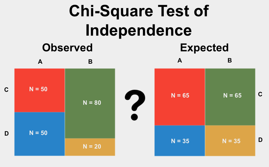
The Chi-Square Test of Independence is used to determine if there is a significant association between two categorical variables. This test helps to understand whether the distribution of one variable differs depending on the category of the other variable.
Steps to Perform a Chi-Square Test of Independence
-
Formulate the Hypotheses:
- Null Hypothesis (H0): Assumes no association between the two variables.
- Alternative Hypothesis (HA): Assumes there is an association between the two variables.
-
Create a Contingency Table:
Construct a table that displays the frequency distribution of the variables. For example:
Category 1 Category 2 Category 3 Group A O11 O12 O13 Group B O21 O22 O23 -
Calculate the Expected Frequencies:
Use the formula:
\( E_{ij} = \frac{( \text{row total} \times \text{column total} )}{ \text{grand total} } \)
For each cell in the table, compute the expected frequency (E).
-
Compute the Chi-Square Statistic:
Use the formula:
\( \chi^2 = \sum \frac{(O_{ij} - E_{ij})^2}{E_{ij}} \)
Where \( O_{ij} \) is the observed frequency and \( E_{ij} \) is the expected frequency.
-
Determine the Degrees of Freedom:
The degrees of freedom (df) is calculated as:
\( df = (r - 1) \times (c - 1) \)
Where \( r \) is the number of rows and \( c \) is the number of columns.
-
Compare to the Critical Value:
Compare the calculated chi-square statistic to the critical value from the chi-square distribution table at the desired significance level (e.g., 0.05).
- If \( \chi^2 \) calculated > critical value, reject the null hypothesis (H0).
- If \( \chi^2 \) calculated ≤ critical value, do not reject the null hypothesis (H0).
Example
Consider a survey investigating the association between gender (Male, Female) and preference for a type of movie (Action, Comedy, Drama). The observed frequencies are:
| Action | Comedy | Drama | |
| Male | 30 | 20 | 10 |
| Female | 25 | 30 | 15 |
Using the chi-square test of independence, we determine if gender is associated with movie preference.
Chi-Square Formula and Calculation
The Chi-Square (\(\chi^2\)) test is a statistical method used to determine if there is a significant association between categorical variables. The test compares the observed frequencies in each category to the frequencies that would be expected if there were no association between the variables.
The formula for the Chi-Square test statistic is:
- \(\chi^2\) = Chi-Square test statistic
- O = Observed frequency
- E = Expected frequency
Steps to Calculate the Chi-Square Statistic
**State the Hypotheses**:
- Null Hypothesis (\(H_0\)): There is no association between the variables.
- Alternative Hypothesis (\(H_A\)): There is an association between the variables.
**Create a Contingency Table**:
- List the observed frequencies of the categories in a table.
**Calculate the Expected Frequencies**:
- Use the formula: \[ E = \frac{(row \, total) \times (column \, total)}{grand \, total} \]
- For each cell in the contingency table, compute the expected frequency.
**Compute the Chi-Square Statistic**:
- For each cell, calculate the Chi-Square component: \[ \frac{(O - E)^2}{E} \]
- Sum all the components to get the Chi-Square statistic.
**Compare to the Critical Value**:
- Determine the degrees of freedom: \[ df = (number \, of \, rows - 1) \times (number \, of \, columns - 1) \]
- Use a Chi-Square distribution table to find the critical value at the desired significance level.
- Compare the calculated Chi-Square statistic to the critical value to determine if you can reject the null hypothesis.
**Example Calculation**:
Consider a study to determine if there is an association between gender (male/female) and preference for a new product (like/dislike).
| Like | Dislike | Total | |
|---|---|---|---|
| Male | 30 | 20 | 50 |
| Female | 20 | 30 | 50 |
| Total | 50 | 50 | 100 |
Expected frequencies are calculated as follows:
Chi-Square statistic calculation:
With 1 degree of freedom (\(df = (2-1)(2-1) = 1\)) and a significance level of 0.05, the critical value from the Chi-Square distribution table is 3.841. Since 6 > 3.841, we reject the null hypothesis and conclude that there is a significant association between gender and product preference.
Examples of Chi-Square Applications
The Chi-Square test is widely used in various fields to determine if there is a significant association between categorical variables. Below are some detailed examples of Chi-Square applications:
-
Example 1: Survey on Ice Cream Preferences
Suppose we surveyed 200 adults and 150 children about their favorite ice cream flavors. The results are summarized in a contingency table:
Chocolate Vanilla Strawberry Others Adults 50 70 45 35 Children 30 50 40 30 - Set Hypotheses:
- Null Hypothesis (H0): There is no association between age group and favorite ice cream flavor.
- Alternative Hypothesis (H1): There is an association between age group and favorite ice cream flavor.
- Calculate Expected Frequencies: Compute expected frequencies for each cell based on the null hypothesis.
- Compute Chi-Square Statistic:
Using the formula:
\( \chi^2 = \sum \frac{(O_i - E_i)^2}{E_i} \)
- Degrees of Freedom:
\( df = (rows - 1) \times (columns - 1) \)
- Find Critical Value or P-Value: Compare the calculated chi-square statistic to the critical value or p-value.
- Draw Conclusion: If the calculated chi-square value is greater than the critical value, reject the null hypothesis.
- Set Hypotheses:
-
Example 2: Genetic Studies
In genetics, a Chi-Square test can be used to determine if the observed frequencies of different genotypes match the expected frequencies based on Mendelian inheritance.
- Observed frequencies are compared to expected frequencies derived from the genetic ratios (e.g., 3:1 for dominant to recessive traits).
- Significant deviations from expected ratios might suggest factors such as genetic linkage or mutation.
-
Example 3: Quality Control
In manufacturing, Chi-Square tests can be used to determine if the number of defects in products from different production lines are independent of the production line.
- Create a contingency table of observed defect counts across different production lines.
- Test if the defect count is independent of the production line, indicating consistent quality control.
These examples illustrate the versatility of the Chi-Square test in analyzing categorical data across various domains.
Comparison Between Z-Test and Chi-Square Test
The Z-test and Chi-Square test are both statistical methods used to test hypotheses, but they are applied in different contexts and have distinct characteristics. Below is a comprehensive comparison between these two tests:
Purpose
- Z-Test: Used to determine if there is a significant difference between sample and population means or between the means of two samples when the population variance is known and the sample size is large.
- Chi-Square Test: Used to test relationships between categorical variables, particularly for independence or goodness of fit. It assesses whether observed frequencies differ from expected frequencies.
Types of Data
- Z-Test: Continuous data that follows a normal distribution.
- Chi-Square Test: Categorical data (nominal or ordinal) that can be summarized in frequency tables.
Hypotheses
- Z-Test:
- Null Hypothesis (\(H_0\)): The sample mean is equal to the population mean or there is no difference between the means of two samples.
- Alternative Hypothesis (\(H_A\)): The sample mean is not equal to the population mean or there is a difference between the means of two samples.
- Chi-Square Test:
- For Goodness of Fit:
- Null Hypothesis (\(H_0\)): The observed frequency distribution matches the expected distribution.
- Alternative Hypothesis (\(H_A\)): The observed frequency distribution does not match the expected distribution.
- For Test of Independence:
- Null Hypothesis (\(H_0\)): The variables are independent.
- Alternative Hypothesis (\(H_A\)): The variables are not independent.
- For Goodness of Fit:
Test Statistics
- Z-Test: The test statistic is the Z-score, calculated as: \[ Z = \frac{\bar{x} - \mu}{\sigma / \sqrt{n}} \] where \(\bar{x}\) is the sample mean, \(\mu\) is the population mean, \(\sigma\) is the population standard deviation, and \(n\) is the sample size.
- Chi-Square Test: The test statistic is the Chi-Square value, calculated as: \[ \chi^2 = \sum \frac{(O - E)^2}{E} \] where \(O\) represents the observed frequency and \(E\) represents the expected frequency.
Assumptions
- Z-Test:
- The data follows a normal distribution.
- The samples are independent.
- The population variance is known (or sample size is large).
- Chi-Square Test:
- The sample is randomly selected.
- Expected frequency in each category should be at least 5.
- The variables are categorical.
Applications
- Z-Test:
- Comparing the sample mean to a known population mean.
- Comparing the means of two independent samples.
- Evaluating the effectiveness of a new drug or treatment.
- Chi-Square Test:
- Determining if there is an association between two categorical variables.
- Testing the goodness of fit for observed data to a theoretical distribution.
- Analyzing survey results to check if distributions of responses differ from expectations.
Key Differences
The Z-test and Chi-Square test are both statistical tools used to test hypotheses, but they are applied in different scenarios and have distinct characteristics. Here are the key differences between them:
- Data Type:
- Z-Test: Used for continuous data. It is suitable when the sample size is large (n > 30) and the data is approximately normally distributed.
- Chi-Square Test: Used for categorical data. It analyzes frequencies or proportions to see if there is an association between variables.
- Purpose:
- Z-Test: Compares sample means to the population mean or compares the means of two samples to see if they are significantly different.
- Chi-Square Test: Tests the independence of two categorical variables or the goodness of fit of an observed distribution to an expected one.
- Hypotheses:
- Z-Test: Null hypothesis states that there is no difference between the means (e.g., \( H_0: \mu_1 = \mu_2 \)).
- Chi-Square Test: Null hypothesis states that there is no association between the variables or that the observed distribution fits the expected distribution (e.g., \( H_0 \): The variables are independent).
- Test Statistic:
- Z-Test: Uses the Z-statistic, which is calculated as \( Z = \frac{\bar{X} - \mu}{\sigma / \sqrt{n}} \), where \( \bar{X} \) is the sample mean, \( \mu \) is the population mean, \( \sigma \) is the standard deviation, and \( n \) is the sample size.
- Chi-Square Test: Uses the Chi-Square statistic, calculated as \( \chi^2 = \sum \frac{(O_i - E_i)^2}{E_i} \), where \( O_i \) is the observed frequency and \( E_i \) is the expected frequency.
- Assumptions:
- Z-Test: Assumes the data is normally distributed and the samples are independent.
- Chi-Square Test: Assumes a sufficiently large sample size for each category (expected frequencies should be at least 5) and that the observations are independent.
- Applications:
- Z-Test: Commonly used in quality control, comparing two means, and hypothesis testing in economics and social sciences.
- Chi-Square Test: Widely used in genetics, survey analysis, marketing research, and any field involving categorical data.
Advantages and Disadvantages
Both the Z-test and Chi-Square test are essential tools in statistical analysis, each with its own advantages and disadvantages. Understanding these can help in choosing the right test for your data.
Advantages of Z-Test
- Simplicity: The Z-test is straightforward and easy to apply, especially when the sample size is large.
- Precision: Z-tests provide precise results for large sample sizes due to the central limit theorem.
- Normal Distribution: Assumes normal distribution of the sample, which is often a valid assumption for many real-world data sets.
Disadvantages of Z-Test
- Sample Size Limitation: Requires large sample sizes to produce accurate results.
- Assumption of Normality: Assumes the data follows a normal distribution, which may not always be the case.
Advantages of Chi-Square Test
- Versatility: Can be used with categorical data, making it suitable for a wide range of applications.
- No Normality Assumption: Does not require the data to follow a normal distribution.
- Goodness of Fit: Useful for testing the goodness of fit and independence between variables.
Disadvantages of Chi-Square Test
- Sample Size Requirement: Requires a sufficiently large sample size to ensure accurate results.
- Expected Frequency: Each category must have an expected frequency of at least 5 to ensure validity.
- Non-Parametric: Being non-parametric, it may have less power compared to parametric tests like the Z-test.
Choosing Between Z-Test and Chi-Square Test
When deciding between the Z-test and Chi-Square test, consider the following:
- Type of Data: Use the Z-test for comparing means of continuous data and the Chi-Square test for categorical data.
- Sample Size: Z-tests are more reliable with large sample sizes, while Chi-Square tests are appropriate for categorical data regardless of sample size, provided each category has a sufficient expected frequency.
- Distribution Assumption: Z-tests assume normal distribution, while Chi-Square tests do not have this requirement.
Both tests are valuable tools, and the choice depends on the nature of your data and the specific hypotheses you are testing.
Common Mistakes and How to Avoid Them
When conducting Z-tests and Chi-square tests, several common mistakes can occur that may affect the validity of the results. Understanding these pitfalls and how to avoid them is crucial for accurate data analysis.
-
Sample Size Issues
- Using Small Sample Sizes: Both Z-tests and Chi-square tests require adequate sample sizes to ensure reliable results. For Chi-square tests, the expected frequency in each category should ideally be 5 or more. Using a small sample size can lead to inaccurate p-values. Solution: Ensure your sample size is sufficiently large before conducting these tests.
- Not Checking for Normality (Z-test): The Z-test assumes that the data is normally distributed, especially in smaller samples. Solution: Verify the normality of your data using normality tests or graphical methods before performing a Z-test.
-
Incorrect Test Application
- Using a Z-test When Variance is Unknown: A common mistake is using a Z-test instead of a T-test when the population variance is unknown. Solution: Use a T-test when the population variance is not known and the sample size is small.
- Misapplying Chi-square Tests: Chi-square tests are for categorical data, not for continuous data. Solution: Ensure that your data is categorical when using a Chi-square test.
-
Data Preparation Mistakes
- Incorrect Data Categorization: For Chi-square tests, improper categorization of data can lead to incorrect conclusions. Solution: Carefully categorize your data and ensure that categories are mutually exclusive and collectively exhaustive.
- Ignoring Assumptions: Both tests have underlying assumptions that must be met. Solution: Review and meet all assumptions for the tests being used to ensure valid results.
-
Interpretation Errors
- Overinterpreting Non-Significant Results: A non-significant result does not prove that there is no effect or association, only that there is not enough evidence to show it. Solution: Report and interpret non-significant results appropriately.
- Confusing Correlation with Causation: Chi-square tests can show association but not causation. Solution: Avoid making causal inferences from Chi-square test results.
By recognizing and avoiding these common mistakes, researchers can ensure more accurate and reliable results in their statistical analyses.

Conclusion
In summary, both the Z-test and Chi-Square test are essential tools in statistical analysis, each with its specific applications and strengths. The Z-test is typically used for hypothesis testing involving the means of a population, particularly when the sample size is large and the population variance is known. It is suitable for continuous data that is normally distributed.
On the other hand, the Chi-Square test is invaluable for analyzing categorical data, allowing researchers to assess relationships between variables or the goodness of fit of observed data to a theoretical distribution. It is particularly useful when dealing with frequencies or counts of data points in different categories.
When choosing between these tests, it is crucial to consider the type of data you are working with and the hypothesis you aim to test. The Z-test is more appropriate for continuous data and comparing population means, while the Chi-Square test excels in examining categorical data and testing relationships or independence between variables.
Both tests, when applied correctly, provide powerful means to validate hypotheses and draw meaningful conclusions from data. By understanding their unique characteristics and appropriate applications, researchers and analysts can make informed decisions that enhance the validity and reliability of their statistical analyses.
Ultimately, the proper application of the Z-test and Chi-Square test contributes significantly to rigorous and accurate scientific research, enabling better decision-making and insights across various fields of study.
Video giải thích về kiểm định Chi-Square. Hướng dẫn chi tiết và dễ hiểu về phương pháp kiểm định quan trọng này trong thống kê.
Kiểm Định Chi-Square
READ MORE:
Video giải thích về kiểm định Z và kiểm định Chi-Square về độc lập. Hướng dẫn chi tiết và dễ hiểu để chọn phương pháp kiểm định phù hợp.
Kiểm Định Z hay Kiểm Định Chi-Square về Độc Lập?


:max_bytes(150000):strip_icc()/Chi-SquareStatistic_Final_4199464-7eebcd71a4bf4d9ca1a88d278845e674.jpg)