Topic example of chi square test of independence: The chi-square test of independence is a powerful statistical tool used to determine if there is a significant association between two categorical variables. This comprehensive guide will walk you through an example of how to conduct this test, interpret the results, and understand its practical applications in various fields such as social sciences, healthcare, and marketing.
Table of Content
- Chi-Square Test of Independence
- Introduction to Chi-Square Test of Independence
- Definition and Purpose
- Hypotheses in Chi-Square Test
- Steps to Perform Chi-Square Test
- Calculating Expected Values
- Calculating Chi-Square Statistic
- Interpreting Results
- Practical Examples
- Performing Chi-Square Test in Software
- Assumptions and Limitations
- Additional Resources
- YOUTUBE: Hướng dẫn và ví dụ về kiểm định Chi-Square cho tính độc lập trong thống kê.
Chi-Square Test of Independence
The Chi-Square test of independence is a statistical test used to determine if there is a significant association between two categorical variables. Here, we present an example to illustrate the process.
Example: Gender and Political Party Preference
Suppose we want to investigate whether gender is associated with political party preference. We collect data from a sample of 500 individuals, summarized in the following contingency table:
| Republican | Democrat | Independent | Total | |
|---|---|---|---|---|
| Male | 120 | 90 | 40 | 250 |
| Female | 110 | 95 | 45 | 250 |
| Total | 230 | 185 | 85 | 500 |
Step 1: Define the Hypotheses
H_0: \text{Gender and political party preference are independent} H_1: \text{Gender and political party preference are not independent}
Step 2: Calculate the Expected Values
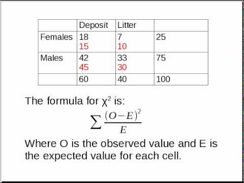
The expected value for each cell is calculated using the formula:
| Republican | Democrat | Independent | |
|---|---|---|---|
| Male | 115 | 92.5 | 42.5 |
| Female | 115 | 92.5 | 42.5 |
Step 3: Calculate \frac{(O-E)^2}{E} for Each Cell
| Republican | Democrat | Independent | |
|---|---|---|---|
| Male | 0.2174 | 0.0676 | 0.1471 |
| Female | 0.2174 | 0.0676 | 0.1471 |
Step 4: Calculate the Test Statistic
The test statistic is calculated as:
Step 5: Determine the p-value and Draw a Conclusion
With 2 degrees of freedom, the p-value associated with the test statistic

READ MORE:
Introduction to Chi-Square Test of Independence
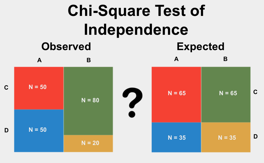
The Chi-Square Test of Independence is a statistical method used to determine if there is a significant association between two categorical variables. This test helps to assess whether the observed frequencies in a contingency table differ significantly from the expected frequencies, which would occur if the variables were independent.
To perform a Chi-Square Test of Independence, follow these steps:
- Formulate the hypotheses:
- Null hypothesis (\(H_0\)): The variables are independent.
- Alternative hypothesis (\(H_a\)): The variables are not independent.
- Construct a contingency table with observed frequencies.
- Calculate the expected frequencies for each cell in the table using the formula:
\[
E = \frac{(\text{row total}) \times (\text{column total})}{\text{grand total}}
\] - Compute the Chi-Square test statistic using the formula:
where \(O\) is the observed frequency and \(E\) is the expected frequency.
\[
\chi^2 = \sum \frac{(O - E)^2}{E}
\] - Determine the degrees of freedom (df) for the test:
where \(r\) is the number of rows and \(c\) is the number of columns.
\[
df = (r - 1) \times (c - 1)
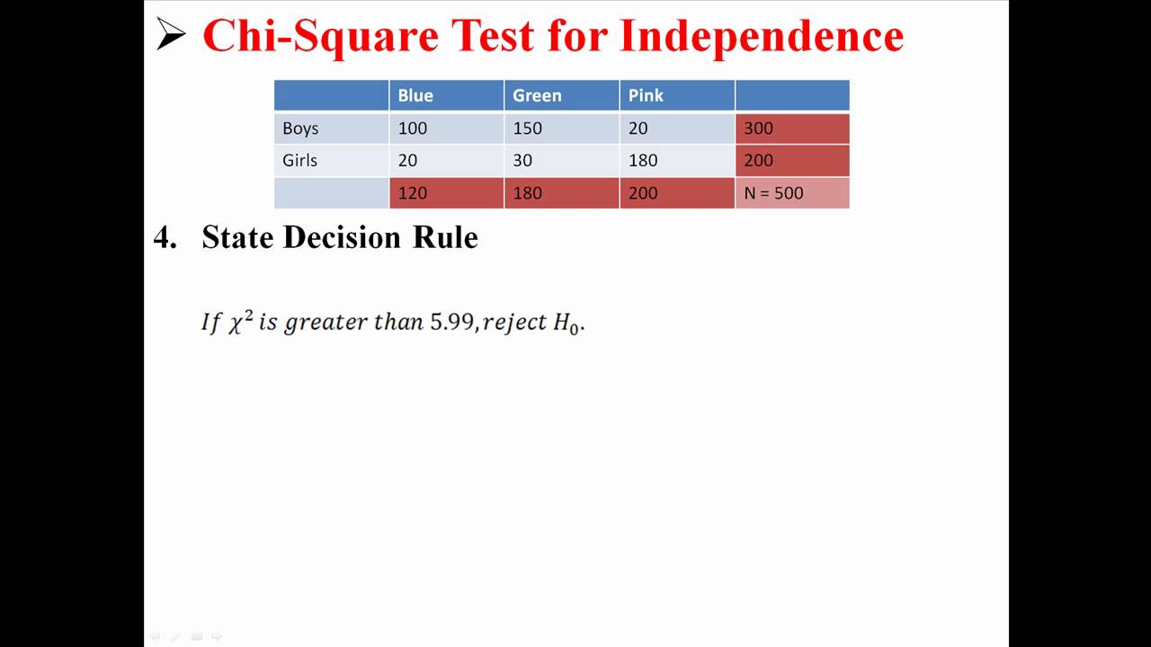
\] - Compare the calculated Chi-Square statistic to the critical value from the Chi-Square distribution table at the desired significance level (e.g., 0.05).
- Make a decision:
- If the Chi-Square statistic is greater than the critical value, reject the null hypothesis (\(H_0\)).
- If the Chi-Square statistic is less than or equal to the critical value, fail to reject the null hypothesis (\(H_0\)).
This test is widely used in research to analyze categorical data and draw meaningful conclusions about the relationship between variables.
Definition and Purpose
The Chi-Square Test of Independence is a statistical method used to determine if there is a significant association between two categorical variables. It assesses whether the observed frequency distribution of a dataset differs from the expected distribution if the variables were independent. This test is widely used in fields like sociology, biology, marketing, and public health to understand relationships between variables.
The purpose of the Chi-Square Test of Independence is to evaluate hypotheses regarding the association between two categorical variables. For instance, it can be used to determine if there is a relationship between gender and voting preference, or between a type of treatment and health outcomes. The test helps researchers make data-driven decisions by providing insights into whether variations in one variable are related to changes in another.
Key steps in conducting the Chi-Square Test of Independence include:
- Formulating Hypotheses: The null hypothesis (\(H_0\)) states that there is no association between the variables, while the alternative hypothesis (\(H_a\)) states that an association exists.
- Constructing a Contingency Table: This table summarizes the observed frequencies of the variables.
- Calculating Expected Frequencies: Expected frequencies are computed assuming the null hypothesis is true.
- Computing the Chi-Square Statistic: The formula used is: \[ \chi^2 = \sum \frac{(O_i - E_i)^2}{E_i} \] where \(O_i\) represents the observed frequency and \(E_i\) represents the expected frequency.
- Determining Degrees of Freedom: The degrees of freedom (df) for the test are calculated using: \[ df = (r-1)(c-1) \] where \(r\) is the number of rows and \(c\) is the number of columns in the contingency table.
- Comparing to Critical Value: The calculated \(\chi^2\) value is compared to a critical value from the Chi-Square distribution table at a specific significance level (\(\alpha\)), typically 0.05.
- Making a Decision: If the \(\chi^2\) value exceeds the critical value, the null hypothesis is rejected, indicating a significant association between the variables.
By following these steps, researchers can effectively use the Chi-Square Test of Independence to uncover potential relationships in categorical data and make informed conclusions.
Hypotheses in Chi-Square Test
The Chi-Square Test of Independence is used to determine if there is a significant association between two categorical variables. The test involves formulating two hypotheses:
- Null Hypothesis (H0): Assumes that there is no relationship between the two categorical variables, meaning they are independent.
- Alternative Hypothesis (Ha): Assumes that there is a relationship between the two categorical variables, meaning they are not independent.
The hypotheses can be formally stated as:
\(H_0: \text{The variables are independent} \)
\(H_a: \text{The variables are not independent} \)
To perform the test, follow these steps:
- Formulate the hypotheses.
- Create a contingency table from the observed frequencies of the variables.
- Calculate the expected frequencies assuming the null hypothesis is true.
- Compute the Chi-Square test statistic using the formula: \[ \chi^2 = \sum \frac{(O_i - E_i)^2}{E_i} \] where \( O_i \) is the observed frequency and \( E_i \) is the expected frequency.
- Determine the degrees of freedom using: \[ df = (r-1) \times (c-1) \] where \( r \) is the number of rows and \( c \) is the number of columns.
- Compare the calculated Chi-Square statistic to the critical value from the Chi-Square distribution table at the desired significance level (e.g., 0.05).
- Make a decision to reject or not reject the null hypothesis based on the comparison.
If the test statistic exceeds the critical value, reject the null hypothesis, indicating there is a significant association between the variables. Otherwise, fail to reject the null hypothesis, suggesting there is no significant association.
Steps to Perform Chi-Square Test
The Chi-Square Test of Independence is used to determine if there is a significant association between two categorical variables. Here are the detailed steps to perform the test:
-
State the Hypotheses
- Null Hypothesis (\(H_0\)): There is no association between the two variables.
- Alternative Hypothesis (\(H_a\)): There is an association between the two variables.
-
Construct a Contingency Table
Create a table that displays the frequency distribution of the variables. Each cell in the table represents the count of occurrences for a specific combination of the variables.
-
Calculate the Expected Frequencies
Use the formula for expected frequencies:
\[
E = \frac{(row\ total \times column\ total)}{grand\ total}
\] -
Compute the Chi-Square Statistic
Apply the Chi-Square formula:
\[
\chi^2 = \sum \frac{(O - E)^2}{E}
\]
where \(O\) is the observed frequency and \(E\) is the expected frequency. -
Determine the Degrees of Freedom
The degrees of freedom (df) are calculated using:
\[
df = (number\ of\ rows - 1) \times (number\ of\ columns - 1)
\] -
Find the P-Value
Compare the Chi-Square statistic to the critical value from the Chi-Square distribution table using the degrees of freedom to find the p-value.
-
Draw a Conclusion
If the p-value is less than the significance level (commonly 0.05), reject the null hypothesis, indicating there is a significant association between the variables.
Calculating Expected Values
The chi-square test of independence assesses whether two categorical variables are associated. One crucial step in this test is calculating the expected values, which are the frequencies we would expect if the null hypothesis were true. Here's a detailed guide on calculating expected values:
- Construct the Contingency Table:
Create a table showing the observed frequencies for each combination of categories of the two variables.
- Calculate the Row and Column Totals:
Sum the observed frequencies for each row and each column to get the marginal totals.
Column 1 Column 2 Total Row 1 O11 O12 Row 1 Total Row 2 O21 O22 Row 2 Total Total Col 1 Total Col 2 Total Grand Total - Compute the Expected Values:
Use the formula \( E = \frac{(\text{Row Total} \times \text{Column Total})}{\text{Grand Total}} \) for each cell.
For example, for cell (1,1):
\( E_{11} = \frac{(\text{Row 1 Total} \times \text{Col 1 Total})}{\text{Grand Total}} \)
- Fill in the Expected Values:
Calculate the expected value for each cell and fill these into a new table matching the structure of the observed frequencies table.
Here's an example to illustrate the process:
Suppose we have the following observed frequencies for two variables:
| Category 1 | Category 2 | Total | |
| Group 1 | 50 | 30 | 80 |
| Group 2 | 20 | 50 | 70 |
| Total | 70 | 80 | 150 |
To calculate the expected value for Group 1, Category 1 (cell (1,1)):
\( E_{11} = \frac{(80 \times 70)}{150} = 37.33 \)
Following this procedure for all cells, we fill in the expected values:
| Category 1 | Category 2 | Total | |
| Group 1 | 37.33 | 42.67 | 80 |
| Group 2 | 32.67 | 37.33 | 70 |
| Total | 70 | 80 | 150 |
These expected values are used in the chi-square test formula to determine if the differences between observed and expected frequencies are significant.
Calculating Chi-Square Statistic
The Chi-Square statistic (\(\chi^2\)) is calculated to determine if there is a significant difference between the expected and observed frequencies in one or more categories. The formula for the Chi-Square statistic is:
\[
\chi^2 = \sum \frac{(O - E)^2}{E}
\]
Where:
- O = Observed frequency
- E = Expected frequency
To perform this calculation, follow these steps:
-
Construct the Contingency Table: Create a table that shows the observed frequencies for each category. For example, if you are analyzing the relationship between gender and preference for a product, your table might look like this:
Product A Product B Male 30 20 Female 25 25 -
Calculate the Expected Frequencies: For each cell in the table, the expected frequency (E) is calculated using the formula:
\[
E = \frac{(Row\ Total \times Column\ Total)}{Grand\ Total}
\]Using the above table, the expected frequency for males preferring Product A would be:
\[
E_{Male, Product\ A} = \frac{(Total\ Males \times Total\ Product\ A)}{Grand\ Total} = \frac{(50 \times 55)}{100} = 27.5
\] -
Compute the Chi-Square Statistic: For each cell in the table, compute the Chi-Square statistic using the formula:
\[
\chi^2 = \sum \frac{(O - E)^2}{E}
\]For example, for males preferring Product A:
\[
\chi^2_{Male, Product\ A} = \frac{(30 - 27.5)^2}{27.5} = \frac{2.5^2}{27.5} = 0.227
\]Repeat this calculation for all cells and sum the results to get the total Chi-Square statistic.
-
Compare to Critical Value: Determine the degrees of freedom (df) for your table, which is calculated as:
\[
df = (number\ of\ rows - 1) \times (number\ of\ columns - 1)
\]For the example table:
\[
df = (2 - 1) \times (2 - 1) = 1
\]Compare your calculated Chi-Square statistic to the critical value from the Chi-Square distribution table at your desired significance level (e.g., 0.05). If the calculated Chi-Square statistic is greater than the critical value, you reject the null hypothesis, indicating a significant association between the variables.
Interpreting Results
Interpreting the results of a Chi-Square Test of Independence involves several steps, from understanding the p-value to making a decision based on the hypothesis. Here is a detailed guide:
P-Value Interpretation
The p-value is a measure that helps determine the significance of your results. It indicates the probability of observing the data, or something more extreme, if the null hypothesis is true. Here's how to interpret the p-value:
- If p ≤ α (the significance level, typically 0.05), reject the null hypothesis. This indicates that there is enough evidence to suggest an association between the variables.
- If p > α, fail to reject the null hypothesis. This means there is not enough evidence to suggest an association between the variables.
For example, in a study testing the independence between gender and political party preference with a p-value of 0.6492 (assuming α = 0.05), we would fail to reject the null hypothesis, indicating no significant association between the two variables.
Decision Making
Based on the p-value and the comparison to your significance level, you can make a statistical decision:
- Reject the Null Hypothesis: If the p-value is less than or equal to the significance level, it suggests that there is a statistically significant association between the two categorical variables. For instance, if you are testing the relationship between seat location and cheating, and the p-value is less than 0.05, you conclude that the seat location is related to cheating behavior.
- Fail to Reject the Null Hypothesis: If the p-value is greater than the significance level, it suggests that there is no statistically significant association between the variables. For example, if you are testing the relationship between dog ownership and cat ownership and the p-value is 0.183 (greater than 0.05), you conclude that there is no significant association between owning dogs and cats.
Real World Conclusion
After deciding whether to reject or fail to reject the null hypothesis, you should state your findings in the context of the real world. Here’s how:
- Explain the implications of your decision. For example, if you rejected the null hypothesis in a study of political affiliation and opinion on a tax reform bill, you might conclude: "There is sufficient evidence to suggest that political affiliation and opinion on the tax reform bill are associated."
- Discuss any limitations or considerations. Note any potential issues such as small expected frequencies or the need for further research.
- Provide practical recommendations or next steps based on your findings.
Example Calculation
To illustrate, let’s consider an example with a chi-square test statistic of 22.152 and degrees of freedom (df) = 2. If the calculated p-value is less than 0.05, we reject the null hypothesis and conclude that the variables are dependent.
Using the formula for the chi-square statistic:
\[
\chi^2 = \sum \frac{(O_i - E_i)^2}{E_i}
\]
Where \(O_i\) are the observed values and \(E_i\) are the expected values. The calculation steps would be:
- Compute the expected values for each cell in the contingency table.
- Calculate the chi-square statistic by summing the squared differences between observed and expected values, divided by the expected values for each cell.
- Determine the p-value using the chi-square distribution with the appropriate degrees of freedom.
For example, if the p-value is 0.000 from our calculation, which is less than 0.05, we reject the null hypothesis and conclude that there is an association between the political affiliation and opinion on the tax reform bill.
By following these steps, you can accurately interpret the results of your Chi-Square Test of Independence and make informed decisions based on your data.
Practical Examples
Below are practical examples of the Chi-Square Test of Independence applied to real-world scenarios.
-
Example 1: Gender and Political Party Preference
In a study, a policy maker wanted to determine if there is an association between gender and political party preference. A sample of 500 voters was surveyed, and the results were tabulated as follows:
Republican Democrat Independent Total Male 120 90 40 250 Female 110 95 45 250 Total 230 185 85 500 The Chi-Square Test of Independence was used to analyze the data. The p-value obtained was 0.649, indicating no significant association between gender and political party preference.
-
Example 2: Seat Location and Cheating
A researcher wanted to find out if there was a relationship between a student's seat location in class and whether they had cheated. The data collected was summarized as follows:
No Yes Total Back 24 8 32 Front 38 8 46 Middle 109 39 148 Total 171 55 226 The Chi-Square Test of Independence yielded a p-value of 0.463. Since this value is greater than the standard alpha level of 0.05, there is no evidence of a relationship between seat location and cheating.
-
Example 3: Dog and Cat Ownership
To determine if there is a relationship between dog and cat ownership, a survey was conducted among students. The results were as follows:
No Cat Yes Cat Total No Dog 183 69 252 Yes Dog 183 89 272 Total 366 158 524 The Chi-Square Test of Independence resulted in a p-value of 0.183. Since this p-value is greater than 0.05, we fail to reject the null hypothesis, suggesting no significant relationship between dog and cat ownership.
Performing Chi-Square Test in Software
Using Minitab
Minitab provides a straightforward process for conducting a Chi-Square Test of Independence:
- Open Minitab and load your data into the worksheet.
- Navigate to Stat > Tables > Chi-Square Test (Two-Way Table in Worksheet).
- Select the columns that contain your categorical data for rows and columns.
- Click OK to perform the test. Minitab will display the observed and expected frequencies, the chi-square statistic, degrees of freedom, and the p-value.
Using R
In R, you can use the chisq.test() function to perform a Chi-Square Test of Independence:
- Install and load the necessary package (if not already available):
install.packages("stats")andlibrary(stats). - Prepare your data as a matrix or table.
- Use the function:
result <- chisq.test(your_data). - Check the output using
summary(result)which includes the chi-square statistic, degrees of freedom, and p-value.
Using Excel
Excel provides built-in functions to perform a Chi-Square Test of Independence:
- Enter your observed data into a table format in the worksheet.
- Calculate the expected frequencies using the formula:
expected = (row total * column total) / grand total. - Use the
CHISQ.TEST(observed_range, expected_range)function to get the p-value. - Optionally, use
CHISQ.INV.RT(probability, degrees_freedom)to find the critical value for comparison.
Using SPSS
SPSS simplifies the process through its GUI:
- Load your dataset into SPSS.
- Go to Analyze > Descriptive Statistics > Crosstabs.
- Place one categorical variable in the Row(s) box and the other in the Column(s) box.
- Click on Statistics and select Chi-Square, then click Continue.
- Click OK to run the test. The output window will display the chi-square statistic, degrees of freedom, and the p-value.
Using Python
In Python, the scipy.stats library provides tools for the Chi-Square Test:
- Install the SciPy package if necessary:
pip install scipy. - Import the library:
from scipy.stats import chi2_contingency. - Prepare your data in a list of lists format.
- Use the function:
chi2, p, dof, expected = chi2_contingency(your_data). - Check the outputs for the chi-square statistic, p-value, degrees of freedom, and expected frequencies.
Assumptions and Limitations
The Chi-Square Test of Independence is a widely used statistical test, but it comes with specific assumptions and limitations that need to be considered for accurate results.
Assumptions
- Independence of Observations: Each observation should be independent of the others. This means that the outcome of one observation does not affect the outcome of another.
- Expected Frequency: The expected frequency in each cell of the contingency table should be at least 5. If this assumption is not met, the test may not be valid.
- Random Sampling: The data should be collected through a process of random sampling to ensure that the sample is representative of the population.
- Data Type: The data should be categorical. This means that the variables being tested should be in nominal or ordinal form.
Limitations
- Sensitivity to Sample Size: The Chi-Square Test is sensitive to the sample size. Larger sample sizes generally provide more reliable results. When sample sizes are too small, the test may not be appropriate, and Fisher's exact test may be used instead.
- Sparse Data: The test can be unreliable if some cells in the contingency table have very low frequencies or are empty. In such cases, alternative tests like Fisher's exact test should be considered.
- Not Robust to Missing Data: The Chi-Square Test does not handle missing data well. If there are missing values, they need to be addressed through methods like data imputation before performing the test.
- Only Tests for Association: The Chi-Square Test only determines if there is an association between the variables; it does not provide information about the strength or direction of the relationship. Measures such as Cramer's V or Phi can be used to assess the strength of the association.
Understanding and adhering to these assumptions and limitations is crucial for correctly applying the Chi-Square Test of Independence and ensuring valid results. Misunderstanding or violating these assumptions can lead to inaccurate conclusions, so it's important to evaluate whether this test is appropriate for your data.
Additional Resources
For those interested in delving deeper into the Chi-Square Test of Independence, the following resources provide comprehensive guides, tutorials, and tools to aid your understanding and application of this statistical test:
-
Online Tutorials and Guides
-
offers a detailed lesson on Chi-Square Test of Independence, including practical examples and step-by-step calculations.
-
provides an easy-to-follow tutorial on performing the Chi-Square Test, complete with sample problems and a clear explanation of the test's conditions and steps.
-
-
Software Implementation
-
explains how to perform the Chi-Square Test in R, including code snippets and interpretation of results. It’s an excellent resource for those looking to use R for their statistical analysis.
-
offers resources and tutorials tailored for clinicians and public health professionals, making complex statistical concepts more accessible.
-
-
Interactive Tools
-
features an online Chi-Square calculator that allows users to input their data and get immediate results without needing specialized software.
-
provides a user-friendly interface to perform Chi-Square tests and other statistical analyses directly through your browser.
-
-
Further Reading
-
offers an in-depth article on the Chi-Square Test, discussing its theoretical background, applications, and limitations in research.
-
provides a comprehensive guide that covers both the basics and advanced aspects of Chi-Square Tests, including assumptions and practical applications.
-
Hướng dẫn và ví dụ về kiểm định Chi-Square cho tính độc lập trong thống kê.
Kiểm định Chi-Square cho Tính Độc lập
READ MORE:
Hướng dẫn chi tiết và ví dụ về kiểm định Chi-Square cho tính độc lập trong phân tích thống kê.
Kiểm định Độc lập bằng Chi-Square


:max_bytes(150000):strip_icc()/Chi-SquareStatistic_Final_4199464-7eebcd71a4bf4d9ca1a88d278845e674.jpg)