Topic chi square test example problems: The Chi-Square Test is a statistical method used to determine if there is a significant association between categorical variables. This article provides example problems to help you understand how to apply the Chi-Square Test, interpret results, and effectively use this powerful tool in various research scenarios. Dive into practical examples and enhance your statistical analysis skills!
Table of Content
- Chi-Square Test Example Problems
- Introduction to Chi-Square Test
- Types of Chi-Square Tests
- Chi-Square Test of Independence
- Chi-Square Goodness of Fit Test
- When to Use a Chi-Square Test
- Calculating Chi-Square Test Statistic
- Examples of Chi-Square Test Applications
- Interpreting Chi-Square Test Results
- Common Mistakes in Chi-Square Test
- Practice Problems and Solutions
- Frequently Asked Questions
- YOUTUBE: Video về Kiểm Tra Chi-Square: Hướng dẫn và ví dụ thực tế về cách áp dụng kiểm tra Chi-Square trong phân tích thống kê.
Chi-Square Test Example Problems
The Chi-Square test is a statistical method used to determine if there is a significant association between categorical variables. Here, we explore example problems using the Chi-Square test for both goodness of fit and independence.
Example 1: Chi-Square Goodness of Fit Test
A shop owner wants to know if the distribution of customers throughout the week matches his expectations.
| Day | Observed Frequency |
|---|---|
| Monday | 50 |
| Tuesday | 60 |
| Wednesday | 40 |
| Thursday | 47 |
| Friday | 53 |
Using the Chi-Square Goodness of Fit Test, he finds that the p-value is 0.359, indicating no significant difference from the expected distribution.
Example 2: Chi-Square Test of Independence
A policy maker wants to determine if gender is associated with political party preference. A survey of 500 voters yields the following:
| Republican | Democrat | Independent | Total | |
|---|---|---|---|---|
| Male | 120 | 90 | 40 | 250 |
| Female | 110 | 95 | 45 | 250 |
| Total | 230 | 185 | 85 | 500 |
The Chi-Square Test of Independence yields a p-value of 0.649, showing no significant association between gender and political party preference.
Example 3: Calculating the Chi-Square Statistic
Consider a dataset where we want to determine if there is an association between political affiliation and opinion on a tax reform bill.
| Opinion | Favor | Indifferent | Opposed | Total |
|---|---|---|---|---|
| Group 1 | 138 | 83 | 64 | 285 |
| Group 2 | 64 | 67 | 84 | 215 |
| Total | 202 | 150 | 148 | 500 |
The Chi-Square statistic is calculated as follows:
\[
\chi^2 = \sum \frac{(O_i - E_i)^2}{E_i} = \frac{(138-115.14)^2}{115.14} + \frac{(83-85.50)^2}{85.50} + \frac{(64-84.36)^2}{84.36} + \frac{(64-86.86)^2}{86.86} + \frac{(67-64.50)^2}{64.50} + \frac{(84-63.64)^2}{63.64} = 22.152
\]
With a p-value less than 0.001, we reject the null hypothesis, concluding that political affiliation and opinion on the tax reform bill are dependent.
Conclusion
The Chi-Square test is a powerful tool for analyzing categorical data and determining relationships between variables. It is widely used in various fields including marketing, biology, and social sciences.

READ MORE:
Introduction to Chi-Square Test
The Chi-Square test, introduced by Karl Pearson in 1900, is a statistical method used to determine if there is a significant association between categorical variables. This test compares the observed frequencies in a contingency table to the frequencies we would expect if the variables were independent.
The formula for the Chi-Square statistic is:
\[ \chi^2 = \sum \frac{(O_i - E_i)^2}{E_i} \]
Where:
- \(O_i\) = Observed frequency
- \(E_i\) = Expected frequency under the null hypothesis
The expected frequency for each category is calculated as:
\[ E_i = \frac{\text{Row Total} \times \text{Column Total}}{\text{Grand Total}} \]
Steps to perform a Chi-Square Test:
- State the null and alternative hypotheses. The null hypothesis typically states that there is no association between the variables.
- Calculate the expected frequencies for each category.
- Compute the Chi-Square statistic using the observed and expected frequencies.
- Determine the degrees of freedom, which is \((\text{number of rows} - 1) \times (\text{number of columns} - 1)\).
- Compare the calculated Chi-Square statistic to the critical value from the Chi-Square distribution table at the desired significance level (e.g., 0.05).
- Make a decision: If the Chi-Square statistic is greater than the critical value, reject the null hypothesis, indicating that there is a significant association between the variables.
The Chi-Square test is a powerful tool for analyzing categorical data and is widely used in various fields such as genetics, marketing, and social sciences.
Types of Chi-Square Tests
The Chi-Square test is a statistical method used to determine if there is a significant association between categorical variables. There are two main types of Chi-Square tests: the Chi-Square Goodness of Fit Test and the Chi-Square Test of Independence. Below, we explore each type in detail.
Chi-Square Goodness of Fit Test
This test is used to determine if a sample data matches a population with a specific distribution. It is particularly useful when you want to see if an observed frequency distribution differs from a theoretical distribution.
- Example: Testing if a die is fair by rolling it multiple times and comparing the observed frequency of each face to the expected frequency, which would be equal for all faces in a fair die.
- Formula: The test statistic is calculated as: \[ \chi^2 = \sum \frac{(O_i - E_i)^2}{E_i} \] where \(O_i\) is the observed frequency and \(E_i\) is the expected frequency.
- Steps:
- Define the null hypothesis (\(H_0\)) and the alternative hypothesis (\(H_1\)).
- Calculate the expected frequencies based on the theoretical distribution.
- Compute the Chi-Square statistic using the formula above.
- Compare the calculated Chi-Square value to the critical value from the Chi-Square distribution table.
- Reject or fail to reject the null hypothesis based on the comparison.
Chi-Square Test of Independence
This test assesses whether two categorical variables are independent of each other. It is commonly used in contingency tables where the frequency of occurrence of different outcomes is tabulated.
- Example: Investigating if gender is associated with political party preference by surveying a group of people and recording their gender and party preference.
- Formula: The test statistic is calculated in a similar way to the Goodness of Fit Test, but with a contingency table: \[ \chi^2 = \sum \frac{(O_{ij} - E_{ij})^2}{E_{ij}} \] where \(O_{ij}\) is the observed frequency in cell \(i,j\) and \(E_{ij}\) is the expected frequency for cell \(i,j\).
- Steps:
- Define the null hypothesis (\(H_0\)) that the variables are independent and the alternative hypothesis (\(H_1\)) that they are not.
- Construct a contingency table from the observed data.
- Calculate the expected frequencies for each cell in the table.
- Compute the Chi-Square statistic using the formula above.
- Compare the calculated Chi-Square value to the critical value from the Chi-Square distribution table.
- Reject or fail to reject the null hypothesis based on the comparison.
Both tests are fundamental tools in statistics, allowing researchers to make inferences about populations based on sample data and to understand the relationships between categorical variables.
Chi-Square Test of Independence
The Chi-Square Test of Independence is used to determine if there is a significant association between two categorical variables. This statistical test compares the observed frequencies in each category of a contingency table to the frequencies that would be expected if there were no association between the variables. Here is a detailed step-by-step guide on how to perform this test:
-
State the Hypotheses
- Null Hypothesis (\(H_0\)): The two variables are independent.
- Alternative Hypothesis (\(H_a\)): The two variables are not independent.
-
Construct the Contingency Table
Collect and tabulate the data into a contingency table, showing the frequency distribution of the variables.
-
Calculate the Expected Frequencies
Use the formula to calculate the expected frequency for each cell in the table:
\[
E = \frac{(R \times C)}{N}
\]where \(R\) is the row total, \(C\) is the column total, and \(N\) is the grand total.
-
Compute the Chi-Square Statistic
Use the formula to calculate the chi-square test statistic:
\[
\chi^2 = \sum \frac{(O - E)^2}{E}
\]where \(O\) is the observed frequency and \(E\) is the expected frequency.
-
Determine the Degrees of Freedom
The degrees of freedom for the test are calculated as:
\[
df = (r-1) \times (c-1)
\]where \(r\) is the number of rows and \(c\) is the number of columns.
-
Find the Critical Value and Compare
Refer to a chi-square distribution table to find the critical value based on the degrees of freedom and significance level (usually 0.05). Compare the computed chi-square statistic to the critical value.
-
Make a Decision
- If the chi-square statistic is greater than the critical value, reject the null hypothesis, indicating a significant association between the variables.
- If the chi-square statistic is less than the critical value, fail to reject the null hypothesis, indicating no significant association.
By following these steps, you can effectively use the Chi-Square Test of Independence to determine if there is a significant relationship between two categorical variables.
Chi-Square Goodness of Fit Test
The Chi-Square Goodness of Fit Test is a statistical method used to determine if a sample data matches a population with a specific distribution. This test is applicable when you have categorical data and want to see if the observed distribution of data differs from the expected distribution based on a hypothesized model.
Steps to Perform a Chi-Square Goodness of Fit Test
- State the Hypotheses:
- \(H_0\): The observed frequencies match the expected frequencies.
- \(H_a\): The observed frequencies do not match the expected frequencies.
- Calculate the Expected Frequencies: Use the formula:
\[
E_i = \frac{n \cdot p_i}{N}
\]
where \(E_i\) is the expected frequency for category \(i\), \(n\) is the total number of observations, \(p_i\) is the expected proportion for category \(i\), and \(N\) is the number of categories. - Compute the Chi-Square Statistic: Use the formula:
\[
\chi^2 = \sum \frac{(O_i - E_i)^2}{E_i}
\]
where \(O_i\) is the observed frequency and \(E_i\) is the expected frequency for category \(i\). - Determine the Degrees of Freedom:
\[
df = k - 1
\]
where \(k\) is the number of categories. - Find the Critical Value: Compare the computed Chi-Square statistic to the critical value from the Chi-Square distribution table at the desired significance level (\(\alpha\)).
- Make a Decision:
- If \(\chi^2\) is greater than the critical value, reject \(H_0\).
- If \(\chi^2\) is less than or equal to the critical value, do not reject \(H_0\).
Example Problem
Consider a dice roll where you expect each number (1 through 6) to appear with equal probability. You roll the dice 60 times, and the observed frequencies are: 8, 10, 9, 12, 11, 10.
- Calculate the Expected Frequencies:
Since there are 60 rolls and 6 outcomes, the expected frequency for each outcome is:
\[
E_i = \frac{60}{6} = 10
\] - Compute the Chi-Square Statistic:
\[
\chi^2 = \sum \frac{(O_i - E_i)^2}{E_i} = \frac{(8-10)^2}{10} + \frac{(10-10)^2}{10} + \frac{(9-10)^2}{10} + \frac{(12-10)^2}{10} + \frac{(11-10)^2}{10} + \frac{(10-10)^2}{10}
\]
\[
\chi^2 = \frac{4}{10} + 0 + \frac{1}{10} + \frac{4}{10} + \frac{1}{10} + 0 = 1
\] - Determine the Degrees of Freedom:
\[
df = 6 - 1 = 5
\] - Find the Critical Value:
For \(\alpha = 0.05\) and \(df = 5\), the critical value from the Chi-Square distribution table is 11.07.
- Make a Decision:
Since \(\chi^2 = 1\) is less than 11.07, we do not reject \(H_0\). Thus, there is no significant difference between the observed and expected frequencies.
When to Use a Chi-Square Test
The Chi-Square test is a statistical method used to determine if there is a significant association between categorical variables. It is particularly useful in the following scenarios:
- Testing for independence: To determine if there is a significant relationship between two categorical variables in a contingency table.
- Goodness of fit: To check if an observed frequency distribution matches an expected distribution based on a theoretical model.
- Homogeneity: To compare the distribution of a categorical variable across different populations.
To conduct a Chi-Square test, follow these steps:
- Formulate the hypotheses:
- Null hypothesis (H0): There is no association between the variables.
- Alternative hypothesis (H1): There is an association between the variables.
- Construct the contingency table: Record the observed frequencies of the variables.
- Calculate the expected frequencies: Use the formula where R is the row total, C is the column total, and N is the grand total.
- Compute the Chi-Square statistic: where O is the observed frequency and E is the expected frequency.
- Determine the degrees of freedom (df): where r is the number of rows and c is the number of columns.
- Compare the Chi-Square statistic to the critical value from the Chi-Square distribution table: Based on the degrees of freedom and the desired significance level (e.g., 0.05), determine if the null hypothesis can be rejected.
The Chi-Square test is a versatile tool in statistics, allowing researchers to test hypotheses about categorical data and determine the relationships between variables effectively.
Calculating Chi-Square Test Statistic
The Chi-Square test statistic is calculated using the formula:
\[\chi^2 = \sum \frac{(O - E)^2}{E}\]
where:
- O is the observed frequency
- E is the expected frequency
Follow these steps to calculate the Chi-Square test statistic:
- Determine the observed frequencies (O) from your data.
- Calculate the expected frequencies (E). For a Chi-Square test of independence, the expected frequency for each cell in a contingency table is calculated as:
\[E = \frac{\text{row total} \times \text{column total}}{\text{grand total}}\]
- Compute the Chi-Square test statistic using the formula mentioned above.
- Compare the computed \(\chi^2\) value to the critical value from the Chi-Square distribution table with the appropriate degrees of freedom to determine the p-value.
- If the p-value is less than the significance level (commonly 0.05), reject the null hypothesis.
Here's an example to illustrate the calculation:
| Category 1 | Category 2 | Category 3 | Total | |
|---|---|---|---|---|
| Group A | 30 | 40 | 50 | 120 |
| Group B | 20 | 60 | 40 | 120 |
| Total | 50 | 100 | 90 | 240 |
First, calculate the expected frequencies for each cell:
| Category 1 | Category 2 | Category 3 | |
|---|---|---|---|
| Group A | \( \frac{120 \times 50}{240} = 25 \) | \( \frac{120 \times 100}{240} = 50 \) | \( \frac{120 \times 90}{240} = 45 \) |
| Group B | \( \frac{120 \times 50}{240} = 25 \) | \( \frac{120 \times 100}{240} = 50 \) | \( \frac{120 \times 90}{240} = 45 \) |
Next, use the Chi-Square formula to calculate the test statistic:
\[
\chi^2 = \sum \frac{(O - E)^2}{E} = \frac{(30-25)^2}{25} + \frac{(40-50)^2}{50} + \frac{(50-45)^2}{45} + \frac{(20-25)^2}{25} + \frac{(60-50)^2}{50} + \frac{(40-45)^2}{45}
\]
Calculating each term:
- \(\frac{(30-25)^2}{25} = 1\)
- \(\frac{(40-50)^2}{50} = 2\)
- \(\frac{(50-45)^2}{45} \approx 0.56\)
- \(\frac{(20-25)^2}{25} = 1\)
- \(\frac{(60-50)^2}{50} = 2\)
- \(\frac{(40-45)^2}{45} \approx 0.56\)
Summing these values gives:
\[
\chi^2 = 1 + 2 + 0.56 + 1 + 2 + 0.56 \approx 7.12
\]
Finally, compare the calculated \(\chi^2\) value to the critical value from the Chi-Square distribution table with the appropriate degrees of freedom (df). The degrees of freedom for this test is calculated as:
\[ df = (number \, of \, rows - 1) \times (number \, of \, columns - 1) \]
For our example, df = (2-1) x (3-1) = 2.
If our significance level is 0.05, the critical value from the Chi-Square distribution table for 2 degrees of freedom is approximately 5.99. Since 7.12 > 5.99, we reject the null hypothesis, indicating there is a significant association between the groups and the categories.
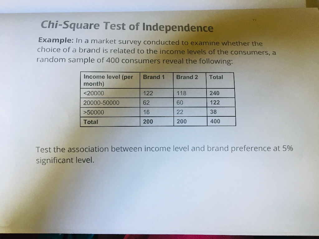
Examples of Chi-Square Test Applications
The Chi-Square test is widely used in various fields to test relationships between categorical variables. Here are some detailed examples of how it can be applied:
1. Chi-Square Test of Independence
This test determines whether there is a significant association between two categorical variables. Let's look at a few examples:
- Voting Preference & Gender: Researchers want to know if gender is associated with political party preference. They survey 500 voters and record their gender and party preference. A Chi-Square Test of Independence can be used to determine if there is a significant relationship between these variables.
- Favorite Color & Favorite Sport: A study surveys 100 people to find out if there is an association between a person's favorite color and their favorite sport. By performing a Chi-Square Test of Independence, researchers can see if these preferences are related.
- Education Level & Marital Status: Data is collected from 2,000 individuals to examine the relationship between their education level and marital status. The Chi-Square test helps determine if there is a significant association between these two variables.
2. Chi-Square Goodness of Fit Test
This test checks if the distribution of a categorical variable matches an expected distribution. Here are some applications:
- Counting Customers: A shop owner wants to know if the number of customers entering the shop each day is uniformly distributed throughout the week. By counting the customers for each day and performing a Chi-Square Goodness of Fit Test, the owner can determine if the actual distribution matches the expected uniform distribution.
- Testing a Die for Fairness: A researcher rolls a die 50 times and records the outcome for each roll. To check if the die is fair, a Chi-Square Goodness of Fit Test is used to see if the observed frequency of each outcome matches the expected frequency of a fair die.
- Distribution of M&M Colors: Suppose we want to check if the color distribution in a bag of M&Ms matches the expected percentages (e.g., 20% yellow, 30% blue, etc.). By counting the M&Ms of each color in a sample bag and using the Chi-Square Goodness of Fit Test, we can test if the observed distribution matches the expected one.
3. Practical Example: Recycling Intervention Study
Consider a study examining the effect of different interventions on household recycling rates:
| Intervention | Outcome | Observed | Expected | (O - E) | (O - E)2 | (O - E)2 / E |
|---|---|---|---|---|---|---|
| Flyer | Recycles | 89 | 84.61 | 4.39 | 19.27 | 0.23 |
| Flyer | Does not recycle | 9 | 13.39 | -4.39 | 19.27 | 1.44 |
| Phone call | Recycles | 84 | 79.43 | 4.57 | 20.88 | 0.26 |
| Phone call | Does not recycle | 8 | 12.57 | -4.57 | 20.88 | 1.66 |
| Control | Recycles | 86 | 94.97 | -8.97 | 80.46 | 0.85 |
| Control | Does not recycle | 24 | 15.03 | 8.97 | 80.46 | 5.35 |
To calculate the Chi-Square test statistic:
\[ \chi^2 = \sum \frac{(O - E)^2}{E} \]
\[ \chi^2 = 0.23 + 1.44 + 0.26 + 1.66 + 0.85 + 5.35 = 9.79 \]
Comparing this to the critical value at a significance level of 0.05 and 2 degrees of freedom (5.99), the test statistic (9.79) is greater, indicating a significant association between intervention type and recycling behavior.
Interpreting Chi-Square Test Results
Interpreting the results of a Chi-Square test involves several key steps to determine if there is a significant association between the variables under study. Here is a detailed guide on how to interpret these results:
-
Determine Statistical Significance: The first step is to compare the p-value to your significance level (typically α = 0.05).
- If the p-value ≤ α, reject the null hypothesis (H0). This indicates that there is a statistically significant association between the variables.
- If the p-value > α, fail to reject the null hypothesis. This suggests there is not enough evidence to conclude that the variables are associated.
-
Examine Observed and Expected Counts: Look at the observed and expected frequencies in each cell of your contingency table.
- Observed Count: The actual frequency observed in the data for each category combination.
- Expected Count: The frequency expected if the null hypothesis is true, calculated based on the marginal totals of the contingency table.
The larger the discrepancy between the observed and expected counts, the larger the contribution to the Chi-Square statistic.
-
Contribution to the Chi-Square Statistic: This is calculated for each cell and shows how much each cell's discrepancy contributes to the overall Chi-Square value.
- Cells with larger contributions are where the observed counts differ most from the expected counts, indicating potential areas of association between the variables.
-
Chi-Square Test Statistic: The Chi-Square statistic (\( \chi^2 \)) itself is calculated by summing the squared differences between observed and expected counts, divided by the expected counts:
\[
\chi^2 = \sum \frac{(O_i - E_i)^2}{E_i}
\]Where \(O_i\) is the observed frequency, and \(E_i\) is the expected frequency for each cell.
-
Degrees of Freedom (df): This is calculated based on the number of categories in your variables:
- For a test of independence: \( \text{df} = (r-1) \times (c-1) \), where \(r\) is the number of rows and \(c\) is the number of columns.
-
Using the Results: If the Chi-Square test is significant, it means that the variables are likely associated. However, it does not indicate the strength or direction of the association. For detailed insights, examine the individual cell contributions and consider follow-up analyses.
In summary, a significant Chi-Square test result tells us that there is an association between the variables. Detailed examination of the observed vs. expected counts and the individual contributions to the Chi-Square statistic provides more specific insights into how the variables might be related.
Common Mistakes in Chi-Square Test
The Chi-Square Test is a powerful tool for statistical analysis, but there are several common mistakes that can lead to incorrect conclusions. Here are some of the most frequent errors:
- Using Percentages Instead of Frequencies: The chi-square test requires data in the form of frequencies (counts) rather than percentages or proportions. Using percentages can distort the results, as the test assumes the data represents actual counts from the population.
- Ignoring Low Expected Frequencies: One key assumption of the chi-square test is that the expected frequency for each cell should be 5 or more. If any expected frequencies are below this threshold, the validity of the test results can be compromised. To address this, you can combine categories or use an alternative test like Fisher's exact test.
- Non-Exhaustive Categories: All possible outcomes should be included in the analysis. Omitting a category can lead to biased results. Ensure that your categories are exhaustive and mutually exclusive.
- Small Sample Sizes: The chi-square test is less reliable with small sample sizes. It is generally recommended to have a larger sample to ensure the robustness of the results.
- Misinterpreting the P-Value: The p-value indicates the probability that the observed differences are due to chance. A low p-value (typically < 0.05) suggests that the observed differences are statistically significant. Misinterpreting this can lead to incorrect conclusions about the relationship between variables.
- Combining Different Tests Incorrectly: Ensure you are using the correct type of chi-square test (Goodness-of-Fit vs. Test of Independence) for your data. Each test has different assumptions and applications.
- Overlooking Assumptions: Chi-square tests have several assumptions, such as the independence of observations and the adequacy of expected frequencies. Failing to meet these assumptions can invalidate the test results.
By being aware of these common mistakes, you can enhance the accuracy and reliability of your chi-square test analyses.
Practice Problems and Solutions
Below are some practice problems to help you understand how to apply the chi-square test in different scenarios, along with detailed solutions.
-
Chi-Square Test of Independence
A researcher wants to determine if there is an association between gender and voting preference. The observed data is as follows:
Gender Republican Democrat Independent Total Male 120 90 40 250 Female 110 95 45 250 Total 230 185 85 500 Solution:
- Calculate the expected frequencies for each cell using the formula: \(E = \frac{(row\ total \times column\ total)}{grand\ total}\).
- Calculate the chi-square test statistic using the formula: \(\chi^2 = \sum \frac{(O - E)^2}{E}\), where O is the observed frequency and E is the expected frequency.
- Determine the degrees of freedom: \(df = (number\ of\ rows - 1) \times (number\ of\ columns - 1)\).
- Compare the calculated chi-square statistic to the critical value from the chi-square distribution table at the desired significance level.
- Make a decision to reject or fail to reject the null hypothesis based on the comparison.
For this example, the p-value is 0.649, which is greater than 0.05, so we fail to reject the null hypothesis. There is no sufficient evidence to suggest an association between gender and voting preference.
-
Chi-Square Goodness of Fit Test
A biologist claims that four different species of deer enter a certain area with equal frequency. The observed data over a week is:
- Species 1: 22
- Species 2: 20
- Species 3: 23
- Species 4: 35
Solution:
- State the null hypothesis \(H_0\): The deer are evenly distributed among the four species.
- Calculate the expected frequencies assuming the null hypothesis is true. If the total number of observations is \(N\), and there are \(k\) categories, then the expected frequency for each category is \(\frac{N}{k}\).
- Compute the chi-square test statistic: \(\chi^2 = \sum \frac{(O - E)^2}{E}\).
- Find the degrees of freedom: \(df = k - 1\).
- Compare the calculated chi-square statistic to the critical value from the chi-square distribution table at the desired significance level.
- Make a decision to reject or fail to reject the null hypothesis based on the comparison.
In this case, the p-value is 0.137, which is greater than 0.05, so we fail to reject the null hypothesis. There is no sufficient evidence to suggest that the distribution of deer is different from what was claimed.
These problems provide a step-by-step approach to applying chi-square tests. Practice with different data sets to strengthen your understanding and proficiency in using this statistical test.
Frequently Asked Questions
-
What is a Chi-Square Test?
A Chi-Square test is a statistical method used to determine if there is a significant association between categorical variables. The most common types are the Chi-Square Goodness of Fit Test and the Chi-Square Test of Independence.
-
What is the difference between the Chi-Square Goodness of Fit Test and the Chi-Square Test of Independence?
- Chi-Square Goodness of Fit Test: Used to determine if a sample data matches a population with a specific distribution. Example: Checking if a die is fair.
- Chi-Square Test of Independence: Used to determine if there is a significant association between two categorical variables. Example: Assessing if voting preference is related to gender.
-
When should I use a Chi-Square Test?
You should use a Chi-Square Test when dealing with categorical variables and you want to test hypotheses about distributions or associations between variables.
-
What are the assumptions of the Chi-Square Test?
- Data should be in the form of frequencies or counts of cases.
- Categories are mutually exclusive.
- Expected frequency in each category should be at least 5.
-
How do I calculate the Chi-Square statistic?
The Chi-Square statistic is calculated using the formula:
\[
X^2 = \sum \frac{(O - E)^2}{E}
\]where \( O \) is the observed frequency and \( E \) is the expected frequency.
-
What does the p-value in a Chi-Square Test indicate?
The p-value indicates the probability that the observed distribution is due to chance. A low p-value (typically < 0.05) suggests that the observed distribution is significantly different from the expected distribution.
-
What are degrees of freedom in a Chi-Square Test?
Degrees of freedom are used to determine the critical value from the Chi-Square distribution table. For the Goodness of Fit Test, it is the number of categories minus one. For the Test of Independence, it is \((\text{number of rows} - 1) \times (\text{number of columns} - 1)\).
-
How do I interpret the results of a Chi-Square Test?
Compare the calculated Chi-Square statistic to the critical value from the Chi-Square distribution table. If the statistic is greater than the critical value, reject the null hypothesis, indicating a significant difference or association.
-
What are some common mistakes when performing a Chi-Square Test?
- Using non-categorical data.
- Ignoring the requirement for expected frequencies to be at least 5.
- Misinterpreting the p-value and critical value comparison.
Video về Kiểm Tra Chi-Square: Hướng dẫn và ví dụ thực tế về cách áp dụng kiểm tra Chi-Square trong phân tích thống kê.
Kiểm Tra Chi-Square
READ MORE:
Video về Cách Thực Hiện Kiểm Tra Chi-Square (Bằng Tay): Hướng dẫn chi tiết và ví dụ thực tế về cách thực hiện kiểm tra Chi-Square thủ công.
Cách... Thực Hiện Kiểm Tra Chi-Square (Bằng Tay)
:max_bytes(150000):strip_icc()/Chi-SquareStatistic_Final_4199464-7eebcd71a4bf4d9ca1a88d278845e674.jpg)