Topic 2 sample chi square test: The 2 Sample Chi-Square Test is a vital tool in statistics, used to determine if there is a significant association between two categorical variables. This test compares observed frequencies with expected frequencies to see if the differences are due to chance or if there is a real effect. It's widely used in various fields to test hypotheses and make data-driven decisions.
Table of Content
- Understanding the 2 Sample Chi-Square Test
- Introduction
- What is a 2 Sample Chi Square Test?
- Applications of 2 Sample Chi Square Test
- Assumptions and Limitations
- Types of Chi-Square Tests
- Steps to Perform a 2 Sample Chi Square Test
- Calculation Example
- Interpretation of Results
- Common Misconceptions
- Advanced Topics
- Graphical Alternatives
- Conclusion
- Additional Resources
- YOUTUBE: Video giới thiệu về Kiểm Định Chi-Square, một phương pháp thống kê quan trọng. Tìm hiểu cách thực hiện và ứng dụng của nó trong phân tích dữ liệu.
Understanding the 2 Sample Chi-Square Test
The 2 Sample Chi-Square Test, also known as the Chi-Square Test of Independence, is a statistical method used to determine whether there is a significant association between two categorical variables in a contingency table. This test compares the observed frequencies of events to the expected frequencies under the null hypothesis of no association between the variables.
Assumptions
- Data should be a random sample from the population.
- Variables under investigation must be categorical.
- Each observation must fall into one unique category (mutually exclusive and exhaustive).
- Expected frequency of each cell in the contingency table should be at least 5 to avoid distortions in the test findings.
Formula
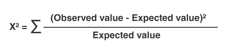
The chi-square statistic (\( \chi^2 \)) is calculated using the formula:
\[
\chi^2 = \sum \frac{(O_i - E_i)^2}{E_i}
\]
where \( O_i \) is the observed frequency and \( E_i \) is the expected frequency.
Steps to Perform the Test
- State the hypotheses: The null hypothesis (\( H_0 \)) states that there is no association between the variables, while the alternative hypothesis (\( H_A \)) states that there is an association.
- Calculate the expected frequencies for each cell in the contingency table.
- Compute the chi-square statistic using the observed and expected frequencies.
- Determine the degrees of freedom (df): \( df = (r - 1) \times (c - 1) \), where \( r \) is the number of rows and \( c \) is the number of columns.
- Compare the calculated chi-square statistic to the critical value from the chi-square distribution table at the chosen significance level (\( \alpha \)).
- Make a decision: If the chi-square statistic is greater than the critical value, reject the null hypothesis; otherwise, fail to reject the null hypothesis.
Examples
Here are some examples of using the 2 Sample Chi-Square Test in real-world scenarios:
- Political Preference by Gender: To determine if there is an association between gender and political party preference, a chi-square test can be applied to survey data.
- Marital Status and Education Level: To investigate whether marital status is related to education level, a chi-square test can analyze data from a random sample of individuals.
- Species Distribution in Ecology: A biologist might use a chi-square test to check if the observed distribution of species in a forest matches the expected distribution.
Limitations and Misconceptions
- The chi-square test cannot establish causality, only association.
- It is not suitable for continuous or ordinal data without appropriate categorization.
- Results can be misleading if expected frequencies are too low, leading to potential Type I or Type II errors.
Interpreting Results
A significant chi-square result indicates an association between the variables, but it's important to consider the practical significance and use measures of effect size, such as Cramer's V or Phi coefficient, to understand the strength of the association.
| Test Statistic (T) | Calculated value of the chi-square statistic |
| Degrees of Freedom (df) | Number of categories minus one |
| Critical Value | Value from chi-square distribution table at chosen significance level |
For further learning, consider exploring statistical textbooks, online courses, and tutorials to deepen your understanding of the chi-square test and its applications.

READ MORE:
Introduction
The 2 sample chi-square test, also known as the chi-square test of independence, is a statistical method used to determine if there is a significant association between two categorical variables. This test is widely used in various fields such as social sciences, marketing, and medical research to examine relationships between categorical data.
The chi-square test compares the observed frequencies in each category to the frequencies that would be expected if there was no association between the variables. The test statistic is calculated using the formula:
\[
\chi^2 = \sum \frac{(O - E)^2}{E}
\]
where \( O \) represents the observed frequency and \( E \) represents the expected frequency under the null hypothesis. The expected frequency is calculated as:
\[
E = \frac{\text{row total} \times \text{column total}}{\text{sample size}}
\]
To perform the test, the value of the chi-square statistic is compared to the critical value from the chi-square distribution with the appropriate degrees of freedom, which is calculated as:
\[
\text{degrees of freedom} = (r - 1) \times (c - 1)
\]
where \( r \) is the number of rows and \( c \) is the number of columns in the contingency table. If the calculated chi-square statistic exceeds the critical value, the null hypothesis is rejected, indicating that there is a significant association between the two variables.
What is a 2 Sample Chi Square Test?
The 2 sample chi-square test, also known as the chi-square test of independence, is a statistical method used to determine if there is a significant association between two categorical variables. This test helps to identify whether the distribution of sample categorical data matches an expected distribution or whether two variables are independent of each other.
- It is applied when you have two nominal variables, and you want to see if they are related.
- The data is often displayed in a contingency table where each cell represents the frequency count of occurrences for combinations of categories.
To perform the test, follow these steps:
- State the Hypotheses:
- Null Hypothesis (H0): The two variables are independent.
- Alternative Hypothesis (HA): The two variables are not independent.
- Collect Data: Create a contingency table summarizing the frequencies of the variables.
- Calculate Expected Frequencies: For each cell in the table, calculate the expected frequency using the formula: \[ E_{ij} = \frac{(Row\ Total_i \times Column\ Total_j)}{Grand\ Total} \]
- Compute the Chi-Square Statistic: Use the formula: \[ \chi^2 = \sum \frac{(O_{ij} - E_{ij})^2}{E_{ij}} \] where \(O_{ij}\) is the observed frequency and \(E_{ij}\) is the expected frequency.
- Determine the Degrees of Freedom: Calculate the degrees of freedom as: \[ df = (rows - 1) \times (columns - 1) \]
- Compare to the Critical Value: Compare the chi-square statistic to the critical value from the chi-square distribution table at the desired significance level (e.g., 0.05). If the chi-square statistic is greater than the critical value, reject the null hypothesis.
This test is widely used in various fields such as marketing, social sciences, and biology to test relationships between categorical variables. It provides insights into the interaction between variables, though it is important to note that it does not imply causation.
In conclusion, the 2 sample chi-square test is a fundamental tool in statistical analysis, offering a way to assess the relationship between two categorical variables, guiding researchers and analysts in their decision-making processes.
Applications of 2 Sample Chi Square Test
The 2 sample chi square test is widely used in various fields to determine if there is a significant association between two categorical variables. Below are some common applications of this statistical test:
- Healthcare: Used to analyze the relationship between treatment types and patient outcomes, such as the effectiveness of different drugs on recovery rates.
- Marketing: Applied to examine the association between customer demographics and purchasing behavior, helping businesses to tailor their marketing strategies effectively.
- Education: Utilized to investigate the correlation between teaching methods and student performance, aiding in the improvement of educational practices.
- Social Sciences: Employed to study the relationship between social factors, such as income level and voting behavior, providing insights into societal trends.
- Quality Control: In manufacturing, it helps in determining whether the defect rates differ between different production lines or shifts.
Overall, the 2 sample chi square test is a versatile tool that provides valuable insights in any scenario where researchers need to understand the association between categorical variables.
Assumptions and Limitations
The 2 Sample Chi Square Test is a powerful tool for analyzing categorical data, but it comes with specific assumptions and limitations. Understanding these is crucial for accurate application and interpretation of the test results.
- Independence of Observations: Each observation must be independent. This means the outcome of one observation should not influence another. This assumption is violated in studies with repeated measures or paired data.
- Sufficient Sample Size: The test is sensitive to small sample sizes. Ideally, each expected frequency in the contingency table should be at least 5 to ensure the validity of the chi-square approximation.
- No Empty Cells: The test can produce misleading results if there are empty cells or cells with very low frequencies. Alternative tests like Fisher's exact test may be more appropriate in these cases.
- Handling of Missing Data: The chi-square test does not handle missing data well. Proper imputation methods should be used to handle missing values before conducting the test.
These assumptions must be met to ensure the accuracy and reliability of the 2 Sample Chi Square Test. When these conditions are not satisfied, the results may not be valid, and alternative statistical methods should be considered.
Types of Chi-Square Tests
Chi-Square tests are statistical methods used to examine the relationships between categorical variables. There are several types of Chi-Square tests, each serving different purposes:
- Pearson’s Chi-Square Test: This test is used to determine if there is a significant association between two categorical variables in a single population. It compares the observed frequencies in a contingency table with the expected frequencies assuming independence between the variables.
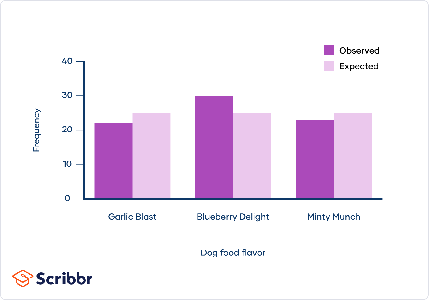
- Chi-Square Goodness of Fit Test: This test is used to assess whether observed categorical data follows an expected distribution. It compares the observed frequencies with the expected frequencies specified by a hypothesized distribution. For example, testing if a die is fair by comparing the observed roll frequencies to the expected frequencies.
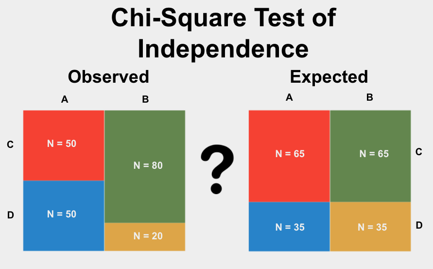
- Chi-Square Test of Independence: This test is used to examine if there is a significant association between two categorical variables in a sample from a population. It compares the observed frequencies in a contingency table with the expected frequencies assuming independence between the variables. For example, analyzing if voting preferences are independent of gender.
Each type of Chi-Square test helps in understanding different aspects of data relationships and is crucial in fields like market research, medicine, and social sciences.
Steps to Perform a 2 Sample Chi Square Test
Performing a 2 Sample Chi Square Test involves several steps. Below is a detailed, step-by-step guide to help you carry out this statistical test:
- Define the Hypotheses
Set up the null hypothesis (\(H_0\)) and the alternative hypothesis (\(H_1\)).
- \(H_0\): The two samples are independent.
- \(H_1\): The two samples are not independent.
- Collect and Organize Data
Gather data and arrange it into a contingency table.
Category 1 Category 2 Total Sample 1 O11 O12 Row 1 Total Sample 2 O21 O22 Row 2 Total Total Column 1 Total Column 2 Total Grand Total - Calculate Expected Frequencies
Use the formula \( E = \frac{(\text{Row Total} \times \text{Column Total})}{\text{Grand Total}} \) to calculate expected frequencies for each cell in the table.
Category 1 Category 2 Sample 1 E11 E12 Sample 2 E21 E22 - Compute Chi-Square Statistic
Calculate the Chi-Square statistic using the formula:
\[
\chi^2 = \sum \frac{(O - E)^2}{E}
\]where \(O\) is the observed frequency and \(E\) is the expected frequency.
- Determine Degrees of Freedom
Calculate the degrees of freedom using the formula:
\[
\text{Degrees of Freedom} = (r - 1) \times (c - 1)
\]where \(r\) is the number of rows and \(c\) is the number of columns.
- Find the P-value
Using the Chi-Square statistic and the degrees of freedom, find the p-value from the Chi-Square distribution table.
- Draw a Conclusion
Compare the p-value to your significance level (\(\alpha\)), typically 0.05. If \(p \leq \alpha\), reject the null hypothesis; otherwise, do not reject the null hypothesis.
Calculation Example
Let's go through a detailed example of performing a 2 Sample Chi-Square Test. We will compare the preferences for two different brands of a product among a sample of consumers.
Step 1: Formulate the Hypotheses
Null Hypothesis (\(H_0\)): There is no significant difference in preferences between the two brands.
Alternative Hypothesis (\(H_1\)): There is a significant difference in preferences between the two brands.
Step 2: Prepare the Contingency Table
Assume we surveyed 100 consumers and obtained the following data:
| Brand | Prefer Brand A | Prefer Brand B | Total |
|---|---|---|---|
| Group 1 | 30 | 20 | 50 |
| Group 2 | 10 | 40 | 50 |
| Total | 40 | 60 | 100 |
Step 3: Calculate the Test Statistic
The Chi-Square test statistic is calculated using the formula:
\[
\chi^2 = \sum \frac{(O_i - E_i)^2}{E_i}
\]
Where \(O_i\) is the observed frequency and \(E_i\) is the expected frequency.
First, we need to calculate the expected frequencies for each cell:
\[
E_{11} = \frac{(50 \times 40)}{100} = 20, \quad E_{12} = \frac{(50 \times 60)}{100} = 30
\]
\[
E_{21} = \frac{(50 \times 40)}{100} = 20, \quad E_{22} = \frac{(50 \times 60)}{100} = 30
\]
Next, we use these expected frequencies to calculate the Chi-Square statistic:
\[
\chi^2 = \frac{(30 - 20)^2}{20} + \frac{(20 - 30)^2}{30} + \frac{(10 - 20)^2}{20} + \frac{(40 - 30)^2}{30}
\]
\[
\chi^2 = \frac{10^2}{20} + \frac{(-10)^2}{30} + \frac{(-10)^2}{20} + \frac{10^2}{30}
\]
\[
\chi^2 = 5 + 3.33 + 5 + 3.33 = 16.66
\]
Step 4: Determine the p-value
To determine the p-value, we need to use the Chi-Square distribution table or a calculator. The degrees of freedom (\(df\)) for our test is:
\[
df = (rows - 1) \times (columns - 1) = (2-1) \times (2-1) = 1
\]
Using a Chi-Square distribution table or calculator, we find the p-value corresponding to \(\chi^2 = 16.66\) and \(df = 1\).
Step 5: Interpret the Results
If the p-value is less than the significance level (e.g., \(\alpha = 0.05\)), we reject the null hypothesis.
In this example, the p-value is much less than 0.05, indicating that there is a significant difference in preferences between the two brands. Therefore, we reject the null hypothesis and conclude that there is a significant difference in preferences between Brand A and Brand B among the surveyed consumers.
Interpretation of Results
Interpreting the results of a 2 Sample Chi-Square Test involves understanding whether the observed association between the variables is statistically significant and what this significance means in the context of the research. Here are the steps to interpret the results:
- Determine Statistical Significance
- Compare the p-value to the chosen significance level (usually α = 0.05).
- If \( p \leq \alpha \), reject the null hypothesis \( H_0 \) and conclude that there is a statistically significant association between the variables.
- If \( p > \alpha \), fail to reject the null hypothesis \( H_0 \) and conclude that there is not enough evidence to support a significant association between the variables.
- Analyze the Chi-Square Statistic
- The chi-square statistic \( \chi^2 \) is calculated as: \[ \chi^2 = \sum \frac{(O_i - E_i)^2}{E_i} \] where \( O_i \) is the observed frequency and \( E_i \) is the expected frequency.
- Compare the calculated \( \chi^2 \) value with the critical value from the chi-square distribution table at the desired significance level and degrees of freedom.
- Interpret Practical Significance
- Even if the test is statistically significant, assess the practical significance by considering the effect size, such as Cramér's V or Phi coefficient, especially in large samples where small differences can be statistically significant.
- Effect size provides insight into the strength of the association between the variables.
- Examine the Contribution to the Chi-Square Statistic
- Identify which cells in the contingency table contribute most to the chi-square statistic by comparing observed and expected counts.
- This helps pinpoint where the largest discrepancies occur, indicating which variable levels have the most significant impact on the association.
For example, if you conducted a study to determine the association between gender and the ability to swim and obtained the following results:
A chi-square test of independence was performed to examine the relation between gender and the ability to swim. The relation between these variables was significant, \( \chi^2 \) (1, N = 84) = 8.9, \( p = 0.0029 \). This indicates that women are more likely than men to be able to swim.
Overall, it is crucial to interpret the results in the context of the research question and hypothesis, considering both statistical and practical significance to make meaningful conclusions about the data.
:max_bytes(150000):strip_icc()/Chi-SquareStatistic_Final_4199464-7eebcd71a4bf4d9ca1a88d278845e674.jpg)
Common Misconceptions
There are several common misconceptions about the 2 Sample Chi-Square Test that can lead to incorrect conclusions. Here are some of the most prevalent ones:
- Misinterpretation of Association as Causation:
The Chi-Square Test can indicate a significant association between variables, but it cannot establish causation. An observed relationship does not imply that one variable causes the other.
- Inappropriate Application to Continuous Data:
The test is designed for categorical data, not continuous data. Applying it to continuous data can lead to misleading results. For continuous variables, consider alternative tests like the t-test or ANOVA.
- Ignoring Expected Frequency Requirements:
Chi-Square tests require that the expected frequency in each cell of the contingency table be at least 5. Ignoring this can invalidate the test results. For small sample sizes, Fisher’s exact test is recommended.
- Assumption of Large Sample Sizes:
While the Chi-Square Test is robust for large samples, it is not limited to them. However, for very small samples, it may not be appropriate, and other methods like Fisher's exact test should be used.
- Overlooking Effect Size:
Statistical significance does not equate to practical significance. It's essential to consider the effect size, such as Cramér's V, to understand the strength of the association between variables.
Understanding these misconceptions can help in correctly applying the 2 Sample Chi-Square Test and accurately interpreting its results.
Advanced Topics
In this section, we explore advanced topics related to the 2 Sample Chi-Square Test, including specific corrections, handling various types of data, and additional statistical tests that can complement the chi-square test.
Yates's Correction for Continuity
Yates's correction for continuity is applied to chi-square tests when dealing with small sample sizes. It adjusts the chi-square formula to account for the discrete nature of categorical data, which can reduce the risk of Type I errors.
- Calculate the expected frequencies for each cell in the contingency table.
- Apply Yates's correction by modifying the formula:
\[
\chi^2 = \sum \frac{(|O - E| - 0.5)^2}{E}
\]
where \( O \) is the observed frequency, and \( E \) is the expected frequency. - Compare the adjusted chi-square value to the critical value from the chi-square distribution table.
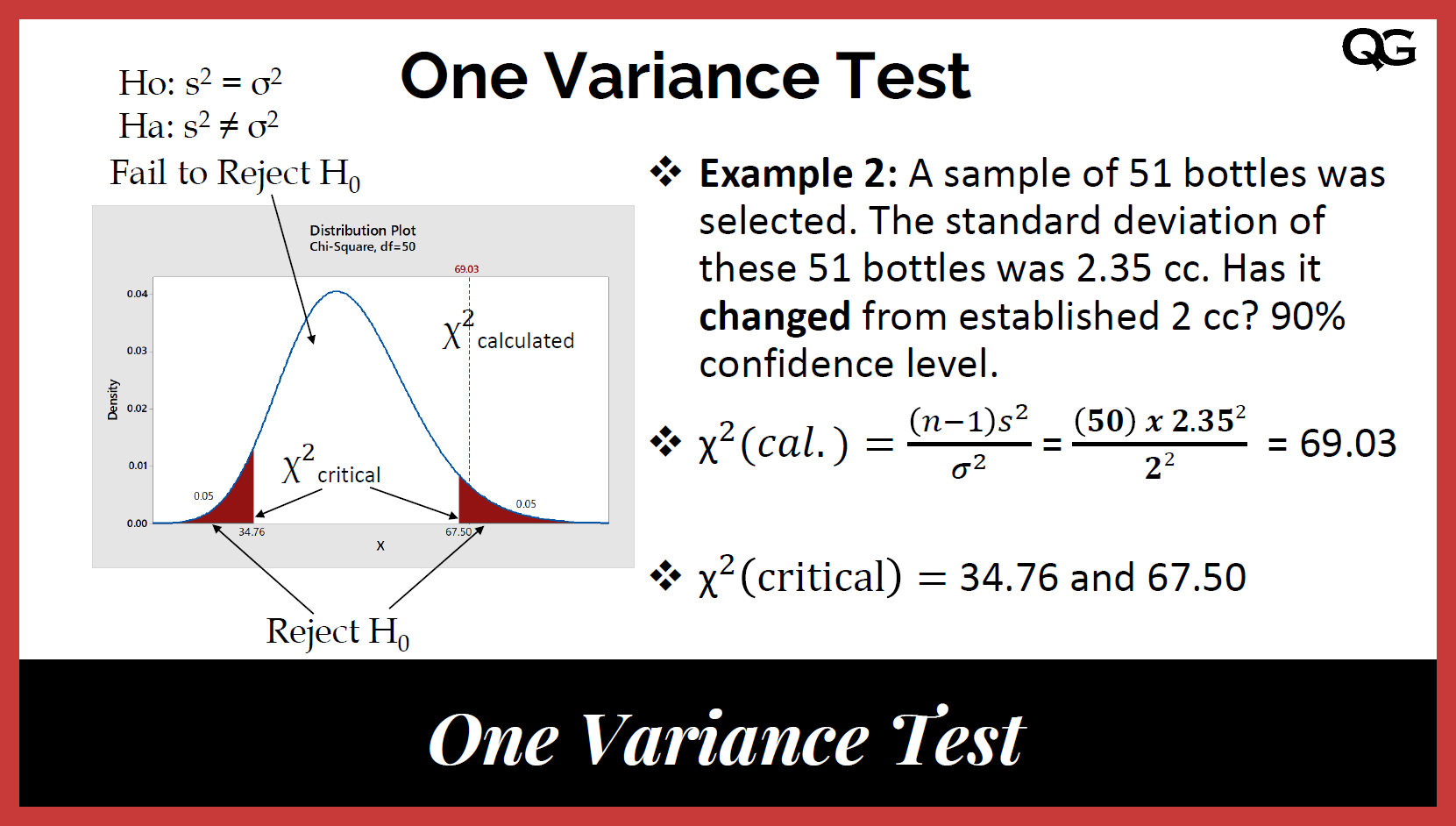
Chi-Square Test for Variance in a Normal Population
This test is used to determine whether a sample variance differs significantly from a known or hypothesized population variance, assuming the population follows a normal distribution.
- Calculate the sample variance \( s^2 \).
- Formulate the null hypothesis \( H_0 \) that the sample variance equals the population variance \( \sigma^2 \).
- Compute the test statistic:
\[
\chi^2 = \frac{(n-1) \cdot s^2}{\sigma^2}
\]
where \( n \) is the sample size. - Compare this test statistic to the critical value from the chi-square distribution with \( n-1 \) degrees of freedom.
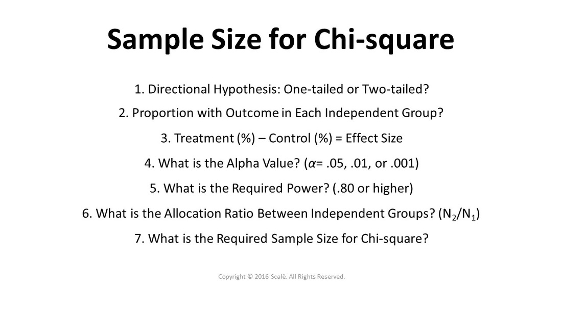
Power Analysis and Effect Size
Power analysis helps determine the sample size required to detect an effect of a given size with a certain degree of confidence. The effect size for a chi-square test can be measured using Cramér's V or the w coefficient.
- Calculate the effect size \( w \):
\[
w = \sqrt{\frac{\chi^2}{n}}
\]
where \( \chi^2 \) is the chi-square statistic, and \( n \) is the total sample size. - Use power analysis formulas or software to determine the required sample size for a given power level (commonly 0.8) and significance level (commonly 0.05).
Combining Chi-Square Distributions
When dealing with multiple independent chi-square variables, their sum also follows a chi-square distribution. This property is useful in meta-analysis or when combining results from different studies.
- Identify the degrees of freedom for each independent chi-square variable.
- Sum the chi-square statistics and their respective degrees of freedom:
\[
\chi^2_{total} = \chi^2_1 + \chi^2_2 + \ldots + \chi^2_k
\]
and
\[
df_{total} = df_1 + df_2 + \ldots + df_k
\]
where \( k \) is the number of independent chi-square variables. - Use the total chi-square statistic and total degrees of freedom to draw conclusions from the combined data.
Extensions to Non-Normal Data
In cases where data do not follow a normal distribution, alternative tests such as the Fisher's Exact Test or logistic regression can be used. These tests are robust to non-normality and can handle small sample sizes more effectively.
- Fisher's Exact Test: Used for small sample sizes and 2x2 tables, providing exact p-values.
- Logistic Regression: Models the relationship between a binary dependent variable and one or more independent variables, offering more flexibility than chi-square tests.
Graphical Alternatives
While the 2 Sample Chi-Square Test is a robust statistical method for analyzing categorical data, there are several graphical alternatives that can provide insightful visual representations of data distributions and relationships. These graphical methods can often highlight trends and differences that may not be immediately obvious from numerical analysis alone.
- Quantile-Quantile Plot (Q-Q Plot)
A Q-Q plot is used to compare the quantiles of two distributions. It is particularly useful for assessing if two data sets come from populations with a common distribution. Points falling approximately along a straight line indicate that the distributions are similar.
Example of creating a Q-Q plot:
# In R qqplot(sample1, sample2, main="Q-Q Plot", xlab="Quantiles of Sample 1", ylab="Quantiles of Sample 2") abline(0, 1) - Bihistogram
A bihistogram displays two histograms back-to-back. This method is useful for comparing the distributions of two groups within the same variable.
Example of creating a bihistogram:
# In R hist(sample1, col=rgb(0,0,1,0.5), xlim=c(min(sample1,sample2),max(sample1,sample2)), main="Bihistogram", xlab="Values") hist(sample2, col=rgb(1,0,0,0.5), add=TRUE) - Tukey Mean-Difference Plot (Bland-Altman Plot)
This plot is used to analyze the agreement between two quantitative measurements. It plots the difference between each pair of observations against their average.
Example of creating a Tukey mean-difference plot:
        # In R
        mean_diff <- (sample1 + sample2) / 2
        diff <- sample1 - sample2
        plot(mean_diff, diff, main="Tukey Mean-Difference Plot", xlab="Mean of Samples", ylab="Difference of Samples")
        abline(h=0, col="red")
Using these graphical methods can complement the findings from a 2 Sample Chi-Square Test, providing a more comprehensive understanding of the data.
Conclusion
The 2 Sample Chi-Square Test is a robust statistical tool used to determine if there is a significant association between two categorical variables. It plays a crucial role in many fields such as social sciences, biology, and market research. By comparing the observed frequencies to the expected frequencies, this test helps researchers understand the relationships within their data.
Key takeaways include:
- Formulating the null hypothesis that there is no association between the variables.
- Calculating the Chi-Square statistic to compare observed and expected values.
- Interpreting the p-value to determine the significance of the results.
The test's simplicity and effectiveness make it a valuable method for analyzing categorical data. However, researchers must be mindful of the assumptions and limitations, such as the need for a sufficiently large sample size and expected frequencies, to ensure accurate results.
In conclusion, the 2 Sample Chi-Square Test remains a fundamental technique for statistical analysis, providing insights that drive data-driven decisions and scientific discoveries.

Additional Resources
Here are some additional resources to help you further understand and perform the 2 Sample Chi-Square Test:
- Online calculators for Chi-Square Tests:
- Further reading and advanced statistical techniques:
- How to perform Chi-Square Tests using different statistical software:
Video giới thiệu về Kiểm Định Chi-Square, một phương pháp thống kê quan trọng. Tìm hiểu cách thực hiện và ứng dụng của nó trong phân tích dữ liệu.
Kiểm Định Chi-Square
READ MORE:
Video về Kiểm Định Độc Lập Chi-Square, một phương pháp thống kê sử dụng cho bảng hai chiều. Tìm hiểu cách thực hiện và ứng dụng của nó trong phân tích dữ liệu.
Kiểm Định Độc Lập Chi-Square (Kiểm Định Chi-Square cho Bảng Hai Chiều)