Topic sample of chi square test: The chi-square test is a powerful statistical tool used to examine relationships between categorical variables. This guide provides a thorough explanation and practical examples of chi-square tests, making it easy to understand and apply in various fields. Learn how to conduct, interpret, and utilize the chi-square test effectively in your research or studies.
Table of Content
- Chi-Square Test: Definition, Formula, and Example
- Introduction to Chi-Square Test
- Understanding Chi-Square Distribution
- Types of Chi-Square Tests
- Steps to Perform Chi-Square Test
- Interpreting Chi-Square Test Results
- Assumptions and Limitations of Chi-Square Test
- Applications of Chi-Square Test in Various Fields
- Chi-Square Test in Statistical Software
- Advanced Topics in Chi-Square Test
- Advanced Topics in Chi-Square Test
- YOUTUBE: Hướng dẫn chi tiết về kiểm định Chi-Square, bao gồm các ví dụ và cách sử dụng phần mềm thống kê.
Chi-Square Test: Definition, Formula, and Example
The Chi-Square test is a statistical method used to determine if there is a significant association between two categorical variables. It is widely used in hypothesis testing to compare observed data with data expected to be obtained according to a specific hypothesis.
Conditions for Chi-Square Test
- The data must be in the form of frequencies or counts of cases.
- All individual observations must be independent of each other.
- The sample size should be sufficiently large, typically at least 50 observations in total.
- Expected frequency in each cell of the table should be at least 5.
Formula
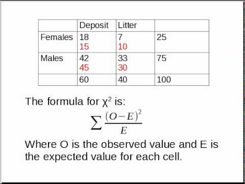
The formula for the Chi-Square statistic is:
\[
\chi^2 = \sum \frac{(O_i - E_i)^2}{E_i}
\]
where \( O_i \) is the observed frequency and \( E_i \) is the expected frequency.
Steps to Perform a Chi-Square Test
- Calculate the expected frequencies: \[ E = \frac{(\text{Row total} \times \text{Column total})}{\text{Grand total}} \]
- Compute the Chi-Square statistic: Using the formula above, calculate the Chi-Square statistic.
- Determine the degrees of freedom (df): \[ df = (\text{number of rows} - 1) \times (\text{number of columns} - 1) \]
- Find the critical value: Use a Chi-Square distribution table to find the critical value for your calculated degrees of freedom and desired significance level (typically 0.05).
- Compare the Chi-Square statistic to the critical value: If the Chi-Square statistic is greater than the critical value, reject the null hypothesis.
Example
Suppose we want to know if gender influences political party preference. We survey 440 voters, and the results are as follows:
| Republican | Democrat | Independent | Total | |
| Male | 100 | 70 | 30 | 200 |
| Female | 140 | 60 | 20 | 220 |
| Total | 240 | 130 | 50 | 440 |
Expected Frequencies
Calculate the expected frequency for each cell:
\[
E_{Male, Republican} = \frac{(200 \times 240)}{440} = 109.09
\]
Similarly, calculate for other cells:
| Republican | Democrat | Independent | Total | |
| Male | 109.09 | 59.09 | 22.73 | 200 |
| Female | 130.91 | 70.91 | 27.27 | 220 |
| Total | 240 | 130 | 50 | 440 |
Chi-Square Calculation
Using the formula:
\[
\chi^2 = \sum \frac{(O_i - E_i)^2}{E_i}
\]
Calculations for each cell are summed to get the Chi-Square statistic:
\[
\chi^2 = \frac{(100 - 109.09)^2}{109.09} + \frac{(70 - 59.09)^2}{59.09} + \ldots = 11.68
\]
Conclusion
Compare the calculated Chi-Square statistic to the critical value from the Chi-Square distribution table. If the calculated value is greater than the critical value, reject the null hypothesis, indicating a significant association between gender and political party preference.

READ MORE:
Introduction to Chi-Square Test
The chi-square test is a statistical method used to determine if there is a significant association between two categorical variables. This test is particularly useful in fields such as social sciences, biology, and marketing, where researchers often deal with categorical data.
There are two main types of chi-square tests:
- Chi-Square Test for Independence: Used to determine if there is a significant association between two categorical variables.
- Chi-Square Test for Goodness of Fit: Used to determine if a sample data matches a population with a specific distribution.
To perform a chi-square test, follow these steps:
- Formulate Hypotheses: Set up the null hypothesis (\(H_0\)) stating that there is no association between the variables, and the alternative hypothesis (\(H_1\)) stating that there is an association.
- Calculate Expected Frequencies: Use the formula \[ E_{ij} = \frac{{\text{row total} \times \text{column total}}}{\text{grand total}} \] to find the expected frequency for each cell in the contingency table.
- Compute the Chi-Square Statistic: Use the formula \[ \chi^2 = \sum \frac{{(O_{ij} - E_{ij})^2}}{E_{ij}} \] where \(O_{ij}\) is the observed frequency and \(E_{ij}\) is the expected frequency.
- Determine Degrees of Freedom: Calculate the degrees of freedom using the formula \[ df = (r-1) \times (c-1) \] where \(r\) is the number of rows and \(c\) is the number of columns.
- Compare with Critical Value: Compare the computed chi-square statistic with the critical value from the chi-square distribution table at the desired significance level (e.g., 0.05). If the statistic exceeds the critical value, reject the null hypothesis.
By following these steps, you can effectively use the chi-square test to analyze categorical data and draw meaningful conclusions about the relationships between variables.
Understanding Chi-Square Distribution
The chi-square distribution is a theoretical distribution that is widely used in statistical tests. It is particularly useful in chi-square tests, where it helps to determine the significance of observed differences or associations in categorical data.
Key characteristics of the chi-square distribution include:
- Non-Negative Values: The chi-square distribution is defined for values greater than or equal to zero. It cannot take negative values.
- Skewed Distribution: The distribution is positively skewed, especially for lower degrees of freedom. As the degrees of freedom increase, the distribution becomes more symmetrical.
- Degrees of Freedom: The shape of the chi-square distribution is determined by its degrees of freedom (df). The degrees of freedom are typically the number of independent values that can vary in the analysis without violating any constraints.
The chi-square distribution is used in the following way:
- Calculating the Chi-Square Statistic: In a chi-square test, the test statistic is calculated using the formula \[ \chi^2 = \sum \frac{{(O_{ij} - E_{ij})^2}}{E_{ij}} \] where \(O_{ij}\) is the observed frequency and \(E_{ij}\) is the expected frequency.
- Determining Degrees of Freedom: The degrees of freedom for a chi-square test are calculated using the formula \[ df = (r-1) \times (c-1) \] for a contingency table, where \(r\) is the number of rows and \(c\) is the number of columns.
- Comparing to Critical Values: The calculated chi-square statistic is compared to the critical value from the chi-square distribution table. The critical value is determined by the chosen significance level (e.g., 0.05) and the degrees of freedom. If the chi-square statistic exceeds the critical value, the null hypothesis is rejected.
The chi-square distribution plays a crucial role in determining the p-value, which helps to decide whether the observed data significantly deviates from the expected data under the null hypothesis. By understanding and applying the chi-square distribution, researchers can make informed decisions about their categorical data analyses.
Types of Chi-Square Tests
Chi-square tests are statistical methods used to determine if there is a significant association between categorical variables. There are two main types of chi-square tests:
Chi-Square Test for Independence
The chi-square test for independence assesses whether two categorical variables are independent of each other. It is often used to examine the relationship between variables in a contingency table.
- Formulate Hypotheses:
- Null hypothesis (\(H_0\)): The variables are independent.
- Alternative hypothesis (\(H_1\)): The variables are not independent.
- Create a Contingency Table: Organize the observed data into a table where rows represent categories of one variable and columns represent categories of the other variable.
- Calculate Expected Frequencies: Use the formula \[ E_{ij} = \frac{{\text{row total} \times \text{column total}}}{\text{grand total}} \] to find the expected frequency for each cell.
- Compute the Chi-Square Statistic: Use the formula \[ \chi^2 = \sum \frac{{(O_{ij} - E_{ij})^2}}{E_{ij}} \] where \(O_{ij}\) is the observed frequency and \(E_{ij}\) is the expected frequency.
- Determine Degrees of Freedom: Calculate the degrees of freedom using the formula \[ df = (r-1) \times (c-1) \] where \(r\) is the number of rows and \(c\) is the number of columns.
- Compare to Critical Value: Compare the chi-square statistic to the critical value from the chi-square distribution table. If the statistic exceeds the critical value, reject the null hypothesis.
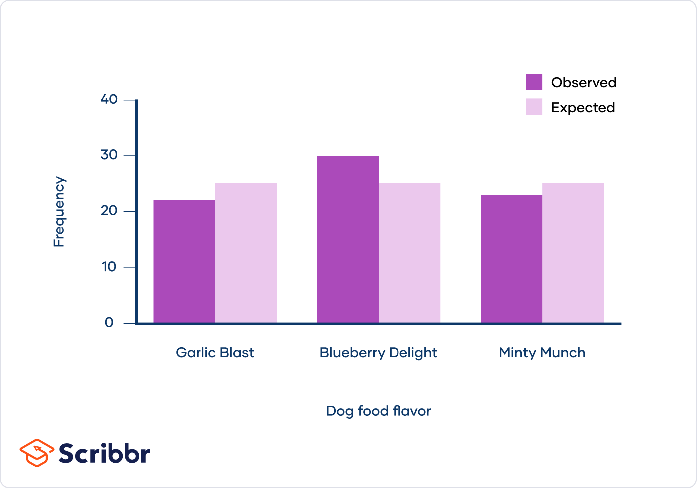
Chi-Square Test for Goodness of Fit
The chi-square test for goodness of fit determines how well a sample data matches a population with a specific distribution. It is used to see if observed frequencies differ from expected frequencies in a single categorical variable.
- Formulate Hypotheses:
- Null hypothesis (\(H_0\)): The observed frequencies match the expected frequencies.
- Alternative hypothesis (\(H_1\)): The observed frequencies do not match the expected frequencies.
- Calculate Expected Frequencies: Determine the expected frequency for each category based on the specified distribution.
- Compute the Chi-Square Statistic: Use the formula \[ \chi^2 = \sum \frac{{(O_i - E_i)^2}}{E_i} \] where \(O_i\) is the observed frequency and \(E_i\) is the expected frequency.
- Determine Degrees of Freedom: Calculate the degrees of freedom using the formula \[ df = n - 1 \] where \(n\) is the number of categories.
- Compare to Critical Value: Compare the chi-square statistic to the critical value from the chi-square distribution table. If the statistic exceeds the critical value, reject the null hypothesis.
By understanding and applying these types of chi-square tests, researchers can analyze categorical data to identify significant associations and distributions.
Steps to Perform Chi-Square Test
The chi-square test is a statistical method used to determine if there is a significant association between categorical variables. Here are the detailed steps to perform a chi-square test:
- Formulate Hypotheses:
- Null hypothesis (\(H_0\)): There is no association between the variables.
- Alternative hypothesis (\(H_1\)): There is an association between the variables.
- Collect and Organize Data: Gather your data and organize it into a contingency table. Each cell in the table represents the frequency count of occurrences for combinations of the categorical variables.
- Calculate Expected Frequencies: Use the formula
\[
E_{ij} = \frac{{\text{row total} \times \text{column total}}}{\text{grand total}}
\]
to calculate the expected frequency for each cell in the contingency table.
For example, if the table has 3 rows and 4 columns, and the grand total is 100, the expected frequency for a cell in the first row and first column is:
\[ E_{11} = \frac{{\text{total of row 1} \times \text{total of column 1}}}{100} \] - Compute the Chi-Square Statistic: Use the formula \[ \chi^2 = \sum \frac{{(O_{ij} - E_{ij})^2}}{E_{ij}} \] where \(O_{ij}\) is the observed frequency and \(E_{ij}\) is the expected frequency. Sum this calculation for all cells in the contingency table.
- Determine Degrees of Freedom: Calculate the degrees of freedom using the formula \[ df = (r-1) \times (c-1) \] where \(r\) is the number of rows and \(c\) is the number of columns in the contingency table.
- Compare to Critical Value: Find the critical value from the chi-square distribution table at the desired significance level (e.g., 0.05) and degrees of freedom. Compare the calculated chi-square statistic to the critical value.
- Make a Decision:
- If the chi-square statistic exceeds the critical value, reject the null hypothesis (\(H_0\)). This indicates a significant association between the variables.
- If the chi-square statistic does not exceed the critical value, do not reject the null hypothesis. This indicates no significant association between the variables.
By following these steps, you can perform a chi-square test to analyze categorical data and determine if there is a significant relationship between variables.
:max_bytes(150000):strip_icc()/Chi-SquareStatistic_Final_4199464-7eebcd71a4bf4d9ca1a88d278845e674.jpg)
Interpreting Chi-Square Test Results
Interpreting the results of a chi-square test involves understanding the statistical significance and the relationship between the variables. Here is a step-by-step guide to interpreting chi-square test results:
- Compare Chi-Square Statistic to Critical Value:
After calculating the chi-square statistic (\(\chi^2\)) and determining the degrees of freedom (\(df\)), compare the \(\chi^2\) value to the critical value from the chi-square distribution table at the chosen significance level (e.g., 0.05).
- Evaluate the P-Value:
The p-value is the probability of observing a chi-square statistic as extreme as, or more extreme than, the value calculated from the sample data, assuming the null hypothesis is true.
- If the p-value is less than the significance level (e.g., \(p < 0.05\)), reject the null hypothesis (\(H_0\)). This indicates a significant association between the variables.
- If the p-value is greater than or equal to the significance level (e.g., \(p \geq 0.05\)), do not reject the null hypothesis. This indicates no significant association between the variables.
- Interpret the Strength and Direction of Association:
The chi-square test itself does not provide information about the strength or direction of the association. However, additional measures such as Cramer's V or the phi coefficient can be used to interpret the strength of the association for contingency tables of different sizes.
- Cramer's V: For tables larger than 2x2, Cramer's V is calculated as \[ V = \sqrt{\frac{\chi^2}{n \cdot \text{min}(r-1, c-1)}} \] where \(n\) is the sample size, \(r\) is the number of rows, and \(c\) is the number of columns.
- Phi Coefficient: For 2x2 tables, the phi coefficient is calculated as \[ \phi = \sqrt{\frac{\chi^2}{n}} \] where \(n\) is the sample size.
- Consider Practical Significance:
While statistical significance indicates whether an association exists, practical significance assesses the real-world relevance of the findings. Consider the effect size, the context of the research, and the implications of the association to determine its practical importance.
- Acknowledge Limitations:
Recognize the limitations of the chi-square test, such as sensitivity to sample size and the requirement for expected frequencies to be sufficiently large. Ensure that these limitations do not undermine the validity of the conclusions drawn from the test.
By carefully interpreting the chi-square test results, researchers can draw meaningful conclusions about the relationships between categorical variables and their implications in various contexts.
Assumptions and Limitations of Chi-Square Test
The chi-square test is a powerful statistical tool, but it comes with certain assumptions and limitations that must be considered to ensure the validity of the results. Here are the key assumptions and limitations:
Assumptions of Chi-Square Test
- Independence of Observations:
Each observation should be independent of the others. This means that the occurrence of one event does not influence the occurrence of another.
- Expected Frequency:
For the chi-square test to be valid, the expected frequency in each cell of the contingency table should be at least 5. If the expected frequency is less than 5 in more than 20% of the cells, the test may not be appropriate.
- Sample Size:
The test requires a sufficiently large sample size to ensure the reliability of the results. Small sample sizes can lead to inaccurate conclusions.
- Categorical Data:
The chi-square test is applicable only to categorical data. Continuous data must be categorized before performing the test.
Limitations of Chi-Square Test
- Sensitivity to Sample Size:
The chi-square test is sensitive to sample size. With large sample sizes, even small differences between observed and expected frequencies can become statistically significant, potentially leading to misleading conclusions.
- Non-Parametric Nature:
As a non-parametric test, the chi-square test does not make assumptions about the distribution of the data. However, this also means it may have less power compared to parametric tests when the data meets parametric assumptions.
- Requires Sufficiently Large Expected Frequencies:
Cells with very small expected frequencies can distort the chi-square statistic, leading to incorrect conclusions. This is particularly problematic in sparse tables with many cells.
- Does Not Indicate Strength or Direction:
The chi-square test can indicate whether an association exists, but it does not provide information about the strength or direction of the association. Additional measures such as Cramer's V or the phi coefficient are needed for this purpose.
- Limited to Frequency Data:
The test is designed for frequency data and may not be appropriate for data that does not fit this structure. Applying the chi-square test to inappropriate data can lead to invalid results.
Understanding these assumptions and limitations is crucial for correctly applying the chi-square test and accurately interpreting its results. By adhering to these guidelines, researchers can ensure the robustness and validity of their statistical analyses.
Applications of Chi-Square Test in Various Fields
The chi-square test is a versatile statistical tool used across various fields to analyze categorical data. Here are some detailed applications of the chi-square test in different domains:
1. Healthcare and Medicine
In healthcare and medicine, the chi-square test is widely used to investigate the association between risk factors and health outcomes.
- Clinical Trials: Evaluating the effectiveness of new treatments by comparing the distribution of outcomes (e.g., cured vs. not cured) between treatment and control groups.
- Epidemiological Studies: Assessing the relationship between exposure to risk factors (e.g., smoking) and the incidence of diseases (e.g., lung cancer).
- Public Health: Analyzing the distribution of health-related behaviors (e.g., vaccination rates) across different populations or regions.
2. Social Sciences
In social sciences, the chi-square test helps researchers understand the relationships between social variables and behaviors.
- Sociology: Examining the association between demographic variables (e.g., age, gender) and social outcomes (e.g., employment status, education level).
- Psychology: Investigating the relationship between categorical variables (e.g., treatment type, response category) in psychological experiments.
- Political Science: Analyzing voting patterns to see if there is a significant association between voter demographics and election outcomes.
3. Business and Marketing
In business and marketing, the chi-square test is used to make data-driven decisions and understand consumer behavior.
- Market Research: Evaluating customer preferences by analyzing the frequency of responses to different products or services.
- Consumer Behavior: Assessing the relationship between demographic factors (e.g., age, income) and purchasing decisions.
- Sales Analysis: Comparing the performance of different sales strategies or promotional campaigns.
4. Education
In education, the chi-square test assists in evaluating teaching methods and student performance.
- Curriculum Assessment: Analyzing the association between different teaching methods and student performance outcomes.
- Student Surveys: Investigating the relationship between student demographics and their responses to educational surveys.
- Program Evaluation: Comparing the effectiveness of various educational programs or interventions.
5. Biology and Environmental Science
In biology and environmental science, the chi-square test helps in studying the relationships between biological and environmental variables.
- Genetics: Testing the association between genetic markers and traits or diseases in populations.
- Ecology: Examining the distribution of species in different habitats to identify significant ecological patterns.
- Environmental Studies: Analyzing the impact of environmental factors (e.g., pollution) on wildlife distribution and health.
The chi-square test's flexibility and applicability across various fields make it a valuable tool for researchers and professionals seeking to understand and interpret relationships within categorical data.
Chi-Square Test in Statistical Software
SPSS
To perform a Chi-Square Test in SPSS, follow these steps:
- Open SPSS and enter your data in a new dataset.
- Click Analyze > Descriptive Statistics > Crosstabs....
- Move the variables of interest into the Row(s) and Column(s) boxes.
- Click the Statistics button and select Chi-square and Phi and Cramer's V.
- Click Continue, then click Cells and select Observed and Expected counts, as well as row, column, and total percentages.
- Click OK to run the test. The results will appear in the SPSS Output Viewer.
R
To perform a Chi-Square Test in R, you can use the following code:
# Create a contingency table
data <- matrix(c(50, 75, 90, 45, 65, 60, 30, 10), nrow=4, byrow=TRUE)
colnames(data) <- c("Snacks", "No Snacks")
rownames(data) <- c("Action", "Comedy", "Family", "Horror")
data <- as.table(data)

# Perform the Chi-Square Test
chi_square_result <- chisq.test(data)
print(chi_square_result)
The output will include the chi-square statistic, degrees of freedom, and p-value.
Excel
To perform a Chi-Square Test in Excel:
- Enter your observed data in a contingency table format.
- Calculate the expected frequencies for each cell using the formula:
= (Row Total * Column Total) / Grand Total - Use the CHISQ.TEST function to compare the observed and expected frequencies:
=CHISQ.TEST(observed_range, expected_range) - Excel will return the p-value for the Chi-Square Test.
Advanced Topics in Chi-Square Test
Yates' Correction for Continuity
When dealing with a 2x2 contingency table, Yates' Correction for Continuity can be applied to the chi-square statistic to reduce the bias in small sample sizes. In SPSS, this is automatically applied when performing a chi-square test on a 2x2 table.
Using Fisher's Exact Test
For small sample sizes or when the assumptions of the chi-square test are violated, Fisher's Exact Test is a preferable alternative. In SPSS, it can be selected in the Crosstabs dialog box under Exact.
Advanced Topics in Chi-Square Test
Yates' Correction for Continuity
Yates' correction for continuity, also known as Yates' chi-squared test, is used to adjust the chi-square statistic when dealing with 2x2 contingency tables. The correction is applied to reduce the chi-square value slightly to account for the discontinuity that arises from using a discrete distribution to approximate a continuous one. The formula for Yates' correction is:
\[
\chi^2 = \sum \frac{(|O - E| - 0.5)^2}{E}
\]
where \( O \) is the observed frequency and \( E \) is the expected frequency. This correction is particularly important when the sample size is small, as it helps to prevent overestimation of statistical significance.
Using Fisher's Exact Test
Fisher's Exact Test is an alternative to the chi-square test when sample sizes are very small. It is used to determine if there are nonrandom associations between two categorical variables. Unlike the chi-square test, Fisher's Exact Test calculates the exact probability of observing the data assuming the null hypothesis is true, without relying on an approximation.
Steps to perform Fisher's Exact Test:
- Construct a 2x2 contingency table with the observed frequencies.
- Calculate the factorial of the row and column totals, and the grand total.
- Use these values to compute the hypergeometric probability for the observed table configuration.
- Sum the probabilities of all tables that have the same marginal totals and are as extreme as or more extreme than the observed table.
Fisher's Exact Test is particularly useful in medical research and other fields where the sample sizes cannot be large enough to satisfy the assumptions of the chi-square test.
Effect Size Measures
To interpret the results of a chi-square test more comprehensively, it is essential to calculate the effect size, which measures the strength of the association between variables. Two common measures of effect size for chi-square tests are Cramer's V and the Phi coefficient.
- Phi Coefficient: Used for 2x2 tables. It is calculated as: \[ \phi = \sqrt{\frac{\chi^2}{n}} \] where \( \chi^2 \) is the chi-square statistic and \( n \) is the total sample size.
- Cramer's V: Used for tables larger than 2x2. It is calculated as: \[ V = \sqrt{\frac{\chi^2}{n(k-1)}} \] where \( k \) is the smaller number of rows or columns in the contingency table.
Chi-Square Test Limitations
While powerful, the chi-square test has several limitations:
- The test requires a sufficiently large sample size; expected frequencies in any cell should ideally be 5 or more to avoid inaccurate results.
- It is sensitive to the size of the sample. With very large samples, even small and practically insignificant differences may appear statistically significant.
- Chi-square tests do not provide information about the direction or strength of the relationship between variables. This is why effect size measures are crucial.
- The test is not appropriate for continuous data unless they are categorized properly.
Hướng dẫn chi tiết về kiểm định Chi-Square, bao gồm các ví dụ và cách sử dụng phần mềm thống kê.
Kiểm Định Chi-Square
READ MORE:
Hướng dẫn chi tiết về kiểm định Chi-Square với các ví dụ đơn giản và dễ hiểu, giúp bạn nắm vững kiến thức thống kê.
Kiểm Định Chi-Square [Giải Thích Đơn Giản]