Chi-Square Test of Goodness of Fit Example: Mastering Statistical Analysis

Chi-Square Test of Goodness of Fit Example

The Chi-Square Test of Goodness of Fit is used to determine if a sample data matches a population with a specific distribution. It helps to evaluate whether the observed frequencies of categories in a sample differ significantly from the expected frequencies, assuming the population distribution is known.

Steps to Perform the Chi-Square Test of Goodness of Fit

State the Hypotheses

- Null Hypothesis ($H_0$): The observed frequency distribution matches the expected frequency distribution.

- Alternative Hypothesis ($H_1$): The observed frequency distribution does not match the expected frequency distribution.
Calculate the Expected Frequencies

For each category, the expected frequency $E_i$ can be calculated as:

$E_i = N \times p_i$

where $N$ is the total number of observations and $p_i$ is the expected proportion for category $i$.
Compute the Chi-Square Statistic

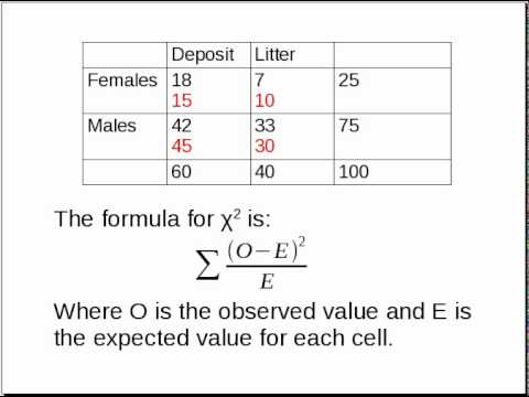
The Chi-Square statistic $ \chi^2 $ is calculated as:

$χ^{2} = \frac{Σ (O_i - E_i)^{2}}{E_i}$

where $O_i$ is the observed frequency for category $i$, and $E_i$ is the expected frequency for category $i$.
Determine the Degrees of Freedom

The degrees of freedom $df$ is calculated as:

$df = k - 1$

where $k$ is the number of categories.
Compare to the Critical Value

Using a Chi-Square distribution table, compare the calculated $ \chi^2 $ value to the critical value with $df$ degrees of freedom at the chosen significance level ($\alpha$, typically 0.05).
Draw a Conclusion

If the calculated $ \chi^2 $ is greater than the critical value, reject the null hypothesis. Otherwise, do not reject the null hypothesis.

Example: Chi-Square Test for Distribution of Colors in M&M's

Suppose a company claims that the color distribution of M&M's in their bags follows the distribution shown below. We want to test if a sample bag of M&M's conforms to this distribution using the Chi-Square Test of Goodness of Fit.

Color	Expected Percentage	Observed Frequency	Expected Frequency	$(O - E)^2 / E$
Red	20%	25	20	1.25
Blue	10%	12	10	0.4
Green	15%	15	15	0
Yellow	30%	30	30	0
Orange	25%	18	25	1.96

Total Chi-Square statistic:

$χ 2 = 1.25 + 0.4 + 0 + 0 + 1.96 = 3.61$

With 4 degrees of freedom ($k-1 = 5-1$), and a significance level of 0.05, the critical value from the Chi-Square distribution table is 9.488.

Since $ \chi^2 = 3.61 $ is less than 9.488, we do not reject the null hypothesis. Therefore, we conclude that the observed distribution of M&M colors does not significantly differ from the expected distribution.

Conclusion

The Chi-Square Test of Goodness of Fit is a powerful statistical tool for evaluating whether observed categorical data conforms to an expected distribution. It is widely used in quality control, survey analysis, and other applications where verifying categorical distributions is crucial.

Chi-Square Test of Goodness of Fit Example

Introduction to the Chi-Square Test of Goodness of Fit

The Chi-Square Test of Goodness of Fit is a statistical test used to determine if there is a significant difference between the observed frequencies and the expected frequencies in one or more categories. This test is particularly useful in categorical data analysis where we compare the observed data distribution against an expected theoretical distribution.

Here’s a detailed step-by-step guide on how to perform the Chi-Square Test of Goodness of Fit:

State the Hypotheses

- Null Hypothesis ($H_0$): The observed frequency distribution matches the expected frequency distribution.

- Alternative Hypothesis ($H_1$): The observed frequency distribution does not match the expected frequency distribution.
Collect and Organize Data

Gather the observed data and determine the expected frequencies based on the population proportions or theoretical distribution. Organize this data into a table for clarity.
Calculate the Expected Frequencies

The expected frequency ($E_i$) for each category is calculated by multiplying the total number of observations ($N$) by the expected proportion ($p_i$) for each category:

$E_i = N \times p_i$
Compute the Chi-Square Statistic

The Chi-Square statistic ($ \chi^2 $) is computed using the formula:

$χ^{2} = \frac{Σ (O_i - E_i)^{2}}{E_i}$

where $O_i$ is the observed frequency and $E_i$ is the expected frequency for each category $i$.
Determine the Degrees of Freedom

The degrees of freedom ($df$) for the Chi-Square Test of Goodness of Fit is calculated as:

$df = k - 1$

where $k$ is the number of categories.
Compare to the Critical Value

Using a Chi-Square distribution table, compare the calculated Chi-Square statistic to the critical value at the chosen significance level ($ \alpha $). If the Chi-Square statistic exceeds the critical value, the null hypothesis is rejected.
Interpret the Results

If the null hypothesis is rejected, it suggests that there is a significant difference between the observed and expected frequencies, indicating that the observed data does not fit the expected distribution well. If the null hypothesis is not rejected, it indicates that the observed distribution fits the expected distribution.

To better understand this test, consider an example where we want to check if a dice is fair. We expect each of the six faces to appear approximately 1/6 of the time over many rolls. The Chi-Square Test of Goodness of Fit helps us determine if the observed frequencies significantly deviate from this expected distribution.

This powerful test is widely used in various fields, including quality control, genetics, and marketing, to validate categorical data assumptions and hypotheses.

Understanding the Chi-Square Statistic

The Chi-Square statistic ($ \chi^2 $) is a measure used in statistical hypothesis testing to assess how expectations compare to actual observed data. It evaluates the difference between the observed frequencies in the data and the frequencies we would expect under a given theoretical distribution.

To understand the Chi-Square statistic, let's break it down step by step:

Observed Frequencies ($O_i$)

These are the actual counts collected from your data. For example, if you roll a dice 60 times, the number of times each face appears is an observed frequency.
Expected Frequencies ($E_i$)

The expected frequencies are the counts you would anticipate if the null hypothesis were true. For instance, if you expect a fair dice, each face should appear $1/6$ of the time. With 60 rolls, each face is expected to appear 10 times.
Calculating the Chi-Square Statistic

The Chi-Square statistic is calculated using the formula:

$χ^{2} = \frac{Σ (O_i - E_i)^{2}}{E_i}$

Where:
- $O_i$ represents the observed frequency for each category $i$.
- $E_i$ represents the expected frequency for each category $i$.
- The summation ($\Sigma$) is over all categories.
Degrees of Freedom ($df$)

The degrees of freedom for a Chi-Square test are calculated as:

$df = k - 1$

where $k$ is the number of categories.
Interpreting the Chi-Square Statistic

To interpret the Chi-Square statistic, compare it to the critical value from the Chi-Square distribution table, given the calculated degrees of freedom and the desired significance level ($ \alpha $). If the calculated $ \chi^2 $ exceeds the critical value, we reject the null hypothesis.

For example, suppose we test a dice for fairness. We roll the dice 60 times and record the observed frequencies as follows:

Face	Observed Frequency ($O_i$)	Expected Frequency ($E_i$)	$(O_i - E_i)^2 / E_i$
1	8	10	0.4
2	12	10	0.4
3	11	10	0.1
4	9	10	0.1
5	10	10	0.0
6	10	10	0.0

The Chi-Square statistic for this data is:

$χ^{2} = 0.4 + 0.4 + 0.1 + 0.1 + 0.0 + 0.0 = 1.0$

With 5 degrees of freedom ($k-1 = 6-1$), we compare this value to the critical value from the Chi-Square distribution table. If our calculated $ \chi^2 $ value is less than the critical value, we fail to reject the null hypothesis, suggesting the dice is fair. Otherwise, we reject the null hypothesis, indicating a significant deviation from expected fairness.

Formulating Hypotheses for the Test

The Chi-Square Test of Goodness of Fit begins with the formulation of two competing hypotheses: the null hypothesis ($H_0$) and the alternative hypothesis ($H_1$). These hypotheses are essential for determining whether the observed data conforms to the expected distribution.

Define the Null Hypothesis ($H_0$)

The null hypothesis ($H_0$) posits that there is no significant difference between the observed frequencies and the expected frequencies. This hypothesis assumes that the observed data fits the expected distribution well. For example, when testing if a dice is fair, the null hypothesis might state:

$H 0 : P (X = 1) = P (X = 2) = ... = P (X = 6) = \frac{1}{6}$
Define the Alternative Hypothesis ($H_1$)

The alternative hypothesis ($H_1$) suggests that there is a significant difference between the observed frequencies and the expected frequencies. This means that the observed data does not fit the expected distribution. Using the dice example, the alternative hypothesis might be:

$H 1 : &exists; i \in {1, 2,... 6}, P (X = i) \neq \frac{1}{6}$
Choosing the Significance Level ($ \alpha $)

The significance level ($ \alpha $) is a threshold set by the researcher to determine whether to reject the null hypothesis. Common significance levels are 0.05, 0.01, and 0.10. The choice of $ \alpha $ affects the critical value against which the Chi-Square statistic is compared.
Setting Up the Decision Rule

The decision rule involves comparing the computed Chi-Square statistic to the critical value from the Chi-Square distribution table. If the Chi-Square statistic exceeds the critical value, we reject the null hypothesis. This rule is based on the degrees of freedom and the chosen significance level. For example:
- If $ \chi^2 $ ≤ $ \chi^2_{\text{critical}} $, Fail to reject $H_0$.
- If $ \chi^2 $ > $ \chi^2_{\text{critical}} $, Reject $H_0$.

By carefully formulating and testing these hypotheses, we can make informed decisions about whether the observed data aligns with the expected distribution or deviates significantly, thereby offering insights into the validity of the underlying assumptions or fairness of the system being tested.

Calculating Expected Frequencies

In the Chi-Square Test of Goodness of Fit, calculating the expected frequencies ($E_i$) is crucial. These expected frequencies are what we anticipate under the null hypothesis, which assumes that the observed data follows a specified distribution. Let's break down the process step by step:

Determine the Total Number of Observations ($N$)

The first step is to find the total number of observed data points. This is simply the sum of all observed frequencies ($O_i$). For instance, if you're analyzing the outcomes of 100 rolls of a dice, $N$ would be 100.
Identify the Expected Proportions ($p_i$)

Next, determine the expected proportion for each category based on the theoretical distribution. For example, if you assume a fair dice, each face should appear with an equal probability of $ \frac{1}{6} $. If different proportions are expected, they should be specified here.
Calculate the Expected Frequencies ($E_i$)

The expected frequency for each category is calculated by multiplying the total number of observations ($N$) by the expected proportion ($p_i$) for that category:

$E_i = N \times p_i$

For example, with 100 dice rolls and each face expected to appear with a probability of $ \frac{1}{6} $, the expected frequency for each face is:

$E_i = 100 \times \frac{1}{6} = 16.67$

Adjust for Different Expected Distributions

If the expected distribution is not uniform, adjust the expected frequencies accordingly. For example, if you expect the dice to be biased such that the probability of rolling a 6 is higher than the other numbers, specify these proportions. Suppose the expected probabilities are $ \frac{1}{12} $ for each face from 1 to 5, and $ \frac{7}{12} $ for face 6. The expected frequencies would be calculated as:

Face	Expected Probability ($p_i$)	Expected Frequency ($E_i$)
1	$\frac{1}{12}$	$100 \times \frac{1}{12} = 8.33$
2	$\frac{1}{12}$	$100 \times \frac{1}{12} = 8.33$
3	$\frac{1}{12}$	$100 \times \frac{1}{12} = 8.33$
4	$\frac{1}{12}$	$100 \times \frac{1}{12} = 8.33$
5	$\frac{1}{12}$	$100 \times \frac{1}{12} = 8.33$
6	$\frac{7}{12}$	$100 \times \frac{7}{12} = 58.33$

These steps ensure that the expected frequencies reflect the theoretical distribution you are testing against. Having accurate expected frequencies is essential for the validity of the Chi-Square Test of Goodness of Fit, as they directly impact the calculation of the Chi-Square statistic and the test's conclusions.

Computing the Chi-Square Statistic

To determine if there is a significant difference between the observed data and the expected frequencies, we compute the Chi-Square statistic ($ \chi^2 $). This statistic quantifies the discrepancy between the observed and expected frequencies. Here’s a step-by-step guide to computing the Chi-Square statistic:

List the Observed and Expected Frequencies

Start by organizing the observed ($ O_i $) and expected ($ E_i $) frequencies for each category into a table. For example, if you have data on the frequency of different colored balls in a sample, it might look like this:

Category	Observed Frequency ($O_i$)	Expected Frequency ($E_i$)
Red	40	30
Blue	35	30
Green	25	30

Apply the Chi-Square Formula

The Chi-Square statistic is calculated using the formula:

$χ^{2} = Σ \frac{(O_i - E_i))^{2}}{E_i}$

Where:
- $O_i$: Observed frequency in category $i$.
- $E_i$: Expected frequency in category $i$.
- $\Sigma$: Summation over all categories.

Calculate Each Component

For each category, compute the component $\frac{(O_i - E_i)^2}{E_i}$ and sum them up:

Category	Observed ($O_i$)	Expected ($E_i$)	$(O_i - E_i)$	$(O_i - E_i)^2$	$\frac{(O_i - E_i)^2}{E_i}$
Red	40	30	10	100	3.33
Blue	35	30	5	25	0.83
Green	25	30	-5	25	0.83

Sum these values to find the Chi-Square statistic:

$χ 2 = 3.33 + 0.83 + 0.83 = 4.99$

Interpret the Chi-Square Statistic

To interpret the Chi-Square statistic, compare it to a critical value from the Chi-Square distribution table, based on your degrees of freedom ($df$) and the chosen significance level ($ \alpha $). The degrees of freedom are calculated as:

$df = k - 1$

Where $ k $ is the number of categories. In our example, with 3 categories, $df = 3 - 1 = 2$.

Once you have the Chi-Square statistic and degrees of freedom, compare your statistic to the critical value in the Chi-Square table. If your calculated $ \chi^2 $ exceeds the critical value, you reject the null hypothesis, indicating a significant difference between the observed and expected frequencies.

Degrees of Freedom in Chi-Square Tests

In Chi-Square tests, the concept of degrees of freedom (df) is crucial for determining the critical value against which the Chi-Square statistic is compared. Degrees of freedom represent the number of independent values or quantities that can vary in an analysis without violating any constraints. Here's a detailed look at how degrees of freedom are calculated and applied in the context of the Chi-Square test of goodness of fit.

Understanding Degrees of Freedom

In statistical terms, degrees of freedom refer to the number of independent pieces of information available to estimate another piece of information. For the Chi-Square test, degrees of freedom are used to determine the shape of the Chi-Square distribution, which influences the critical value needed to assess the significance of the test statistic.
Calculating Degrees of Freedom for Goodness of Fit

For the Chi-Square test of goodness of fit, the degrees of freedom are calculated using the formula:

$df = k - 1$

Where:
- k: The number of categories or distinct groups in your data.
This formula arises because, with $k$ categories, the frequencies in $k-1$ of them are independent. The last frequency is constrained to ensure that the total sum of frequencies equals the sample size. For example, if there are 6 categories (like 6 faces of a die), the degrees of freedom would be $6 - 1 = 5$.
Application in Chi-Square Tests

Once the degrees of freedom are calculated, they are used in conjunction with the Chi-Square statistic to determine the p-value or to compare against a critical value from the Chi-Square distribution table. This comparison helps decide whether to reject the null hypothesis. The critical value depends on the degrees of freedom and the desired level of significance (usually 0.05 or 5%).

For instance, if your Chi-Square statistic is 4.99 with 2 degrees of freedom at a 0.05 significance level, you would check the Chi-Square distribution table to find the critical value for 2 degrees of freedom, which is approximately 5.99. Since 4.99 is less than 5.99, you would not reject the null hypothesis in this case.

Example Calculation

Consider an example where you have a dataset with the following observed and expected frequencies:

Category	Observed Frequency ($O_i$)	Expected Frequency ($E_i$)
A	20	15
B	30	25
C	50	60

Here, there are 3 categories. Using the formula $df = k - 1$, the degrees of freedom are $3 - 1 = 2$. With 2 degrees of freedom, you can now refer to the Chi-Square distribution table to find the critical value for your test.

Conclusion

Understanding and correctly calculating the degrees of freedom are essential for accurately interpreting the results of a Chi-Square test of goodness of fit. It ensures that the test provides valid conclusions about the fit of the observed data to the expected distribution.

Critical Values and Decision Making

The critical value in a chi-square test of goodness of fit is a threshold that determines whether the observed data significantly deviates from the expected data under the null hypothesis. To make a decision about rejecting or failing to reject the null hypothesis, follow these steps:

Determine the significance level (α): Commonly used significance levels are 0.05, 0.01, and 0.10. The significance level represents the probability of rejecting the null hypothesis when it is actually true.
Find the degrees of freedom (df): The degrees of freedom for the chi-square test of goodness of fit is calculated as the number of categories minus one (df = k - 1), where k is the total number of categories.
Use the chi-square distribution table: Locate the critical value corresponding to the chosen significance level and the calculated degrees of freedom from a chi-square distribution table.
Compare the chi-square statistic to the critical value:
- If the calculated chi-square statistic is greater than the critical value, reject the null hypothesis.
- If the calculated chi-square statistic is less than or equal to the critical value, fail to reject the null hypothesis.

Here's a detailed example to illustrate the process:

Suppose we are testing whether a six-sided die is fair. The null hypothesis (H₀) states that each face of the die has an equal probability of landing face up.
We roll the die 60 times and observe the following frequencies: 8, 9, 10, 11, 12, and 10 for faces 1 through 6, respectively.
The expected frequency for each face, assuming the die is fair, is 60 / 6 = 10.
We calculate the chi-square statistic using the formula: \[ \chi^2 = \sum \frac{(O_i - E_i)^2}{E_i} \] where $O_i$ is the observed frequency and $E_i$ is the expected frequency for each category.
For our data, the chi-square statistic is: \[ \chi^2 = \frac{(8-10)^2}{10} + \frac{(9-10)^2}{10} + \frac{(10-10)^2}{10} + \frac{(11-10)^2}{10} + \frac{(12-10)^2}{10} + \frac{(10-10)^2}{10} = 0.4 + 0.1 + 0 + 0.1 + 0.4 + 0 = 1 \]
With 5 degrees of freedom (df = 6 - 1) and a significance level of 0.05, we refer to the chi-square distribution table and find the critical value is 11.070.
Since the calculated chi-square statistic (1) is less than the critical value (11.070), we fail to reject the null hypothesis. There is no significant evidence to suggest that the die is not fair.

Interpreting the Results of the Test

Interpreting the results of the chi-square test of goodness of fit involves understanding whether the observed data matches the expected data under the null hypothesis. Follow these steps to interpret the results:

Calculate the chi-square statistic: Compute the chi-square statistic using the formula: \[ \chi^2 = \sum \frac{(O_i - E_i)^2}{E_i} \] where $O_i$ represents the observed frequency and $E_i$ represents the expected frequency for each category.
Determine the degrees of freedom (df): The degrees of freedom are calculated as the number of categories minus one (df = k - 1), where k is the total number of categories.
Find the critical value: Use a chi-square distribution table to find the critical value corresponding to your chosen significance level (α) and the calculated degrees of freedom.
Compare the chi-square statistic to the critical value:
- If the chi-square statistic is greater than the critical value, reject the null hypothesis.
- If the chi-square statistic is less than or equal to the critical value, fail to reject the null hypothesis.
Draw a conclusion:
- If the null hypothesis is rejected, it suggests that there is a significant difference between the observed and expected frequencies. This means that the observed data does not fit the expected distribution.
- If the null hypothesis is not rejected, it suggests that there is no significant difference between the observed and expected frequencies. This means that the observed data fits the expected distribution.

Let's consider an example for better understanding:

Suppose we are testing whether a die is fair. The null hypothesis (H₀) states that each face of the die has an equal probability of landing face up.
We roll the die 60 times and observe the following frequencies: 8, 9, 10, 11, 12, and 10 for faces 1 through 6, respectively.
The expected frequency for each face, assuming the die is fair, is 60 / 6 = 10.
We calculate the chi-square statistic as: \[ \chi^2 = \frac{(8-10)^2}{10} + \frac{(9-10)^2}{10} + \frac{(10-10)^2}{10} + \frac{(11-10)^2}{10} + \frac{(12-10)^2}{10} + \frac{(10-10)^2}{10} = 0.4 + 0.1 + 0 + 0.1 + 0.4 + 0 = 1 \]
With 5 degrees of freedom (df = 6 - 1) and a significance level of 0.05, the critical value from the chi-square distribution table is 11.070.
Since the calculated chi-square statistic (1) is less than the critical value (11.070), we fail to reject the null hypothesis.
Conclusion: There is no significant evidence to suggest that the die is not fair. The observed frequencies fit the expected distribution of a fair die.

Examples of Chi-Square Test of Goodness of Fit

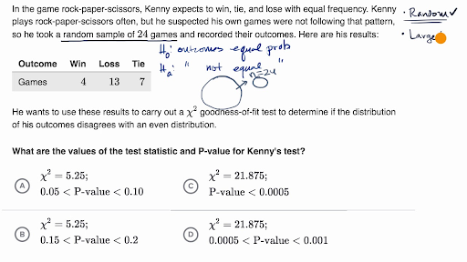
The Chi-Square test of goodness of fit is used to determine whether the observed frequency distribution of a categorical variable matches an expected distribution. Here are detailed examples to illustrate this test:

Example 1: M&M's Color Distribution

Consider a bag of M&M's with the colors red, orange, yellow, green, blue, and brown. We want to test if these colors are equally distributed in a bag.

Hypotheses:
- Null hypothesis ($H_0$): The colors are equally distributed ($p_1 = p_2 = p_3 = p_4 = p_5 = p_6 = \frac{1}{6}$).
- Alternative hypothesis ($H_1$): The colors are not equally distributed.
Observed Frequencies: Suppose we have a sample of 600 M&M's with the following counts:
- Red: 50
- Orange: 147
- Yellow: 46
- Green: 103
- Blue: 212
- Brown: 42
Expected Frequencies: If the colors are equally distributed, we expect each color to have $ \frac{600}{6} = 100 $ M&M's.
Calculate Chi-Square Statistic: The formula for the Chi-Square statistic is: \[ \chi^2 = \sum \frac{(O_i - E_i)^2}{E_i} \] where $O_i$ is the observed frequency and $E_i$ is the expected frequency.
- Red: $ \frac{(50 - 100)^2}{100} = 25 $
- Orange: $ \frac{(147 - 100)^2}{100} = 22.09 $
- Yellow: $ \frac{(46 - 100)^2}{100} = 29.16 $
- Green: $ \frac{(103 - 100)^2}{100} = 0.09 $
- Blue: $ \frac{(212 - 100)^2}{100} = 125.44 $
- Brown: $ \frac{(42 - 100)^2}{100} = 33.64 $
The Chi-Square statistic is $ \chi^2 = 25 + 22.09 + 29.16 + 0.09 + 125.44 + 33.64 = 235.42 $.
Degrees of Freedom: The degrees of freedom ($df$) for this test is $k - 1 = 6 - 1 = 5$, where $k$ is the number of categories.
Determine the p-value: Using a Chi-Square distribution table or calculator, we find the p-value for $ \chi^2 = 235.42 $ with 5 degrees of freedom. The p-value is extremely small, much less than the common significance level of 0.05.
Conclusion: Since the p-value is very small, we reject the null hypothesis. This suggests that the colors are not equally distributed in the bag of M&M's.

Example 2: Customer Distribution Across Weekdays

A shop owner claims that an equal number of customers visit the shop each weekday. To test this, an independent researcher records the number of customers over a week.

Hypotheses:
- Null hypothesis ($H_0$): The number of customers is the same each day.
- Alternative hypothesis ($H_1$): The number of customers varies by day.
Observed Frequencies: The counts are as follows:
- Monday: 50
- Tuesday: 60
- Wednesday: 40
- Thursday: 47
- Friday: 53
Expected Frequencies: If customers are equally distributed, the expected count for each day is $ \frac{250}{5} = 50 $.
Calculate Chi-Square Statistic:
- Monday: $ \frac{(50 - 50)^2}{50} = 0 $
- Tuesday: $ \frac{(60 - 50)^2}{50} = 2 $
- Wednesday: $ \frac{(40 - 50)^2}{50} = 2 $
- Thursday: $ \frac{(47 - 50)^2}{50} = 0.18 $
- Friday: $ \frac{(53 - 50)^2}{50} = 0.18 $
The Chi-Square statistic is $ \chi^2 = 0 + 2 + 2 + 0.18 + 0.18 = 4.36 $.
Degrees of Freedom: $df = 5 - 1 = 4$.
Determine the p-value: For $ \chi^2 = 4.36 $ with 4 degrees of freedom, the p-value is approximately 0.359.
Conclusion: Since the p-value is greater than 0.05, we fail to reject the null hypothesis. There is no significant evidence to suggest that the number of customers differs across the weekdays.

Common Applications of the Test

The Chi-Square Test of Goodness of Fit is a versatile tool used across various fields to determine if observed data matches expected distributions. Here are some common applications:

Biology: Researchers often use this test to analyze the distribution of different species in an environment. For instance, if a biologist wants to see if four species of deer are equally distributed in a forest, they would use the Chi-Square Test to compare observed counts with expected equal distribution.
Psychology: In psychological studies, the test can determine if the frequency of responses fits expected theoretical distributions. For example, if a psychologist hypothesizes that people will choose among four categories of responses equally, they can use the test to validate this hypothesis.
Marketing: Companies use the Chi-Square Test to evaluate consumer preferences. For example, a business might test whether the observed frequency of product choices aligns with expected preferences based on market research.
Healthcare: In clinical trials, the test helps determine if the distribution of patients' responses to different treatments fits the expected distribution. For instance, comparing the effectiveness of a new drug against a placebo.
Education: Educators use this test to analyze whether students' performance on different sections of a test matches the expected performance levels. This can help in identifying biases in test questions.

Overall, the Chi-Square Test of Goodness of Fit is crucial for researchers and analysts to validate hypotheses about categorical data distributions across various disciplines.

Advantages and Limitations of the Chi-Square Test

The Chi-Square test is a widely used statistical tool, especially for categorical data analysis. Understanding its advantages and limitations can help researchers use it more effectively and interpret the results accurately.

Advantages of the Chi-Square Test

Robustness in Data Distribution: The Chi-Square test does not assume a normal distribution of data, making it suitable for a wide range of datasets.
Ease of Calculation: The test is relatively simple to compute, often involving straightforward arithmetic operations.
Versatility: It can handle data from two or more group studies, making it flexible for various research designs.
Non-parametric Nature: Since it does not rely on parametric assumptions, it is useful for data that do not meet these criteria.
Informative: The test provides insights into the relationship between categorical variables, helping in understanding patterns and associations.

Limitations of the Chi-Square Test

Sample Size Requirements: The test requires a sufficiently large sample size. Each expected cell frequency should be at least 5 to ensure reliable results.
Cell Count Restrictions: It can become complex and less reliable when the contingency table has many cells (over 20), as it may violate the expected frequency assumptions.
Sensitivity to Sample Size: The test can be overly sensitive to large sample sizes, leading to significant results for trivial associations.
Difficulty with Sparse Data: When data are sparse or contain cells with very low frequencies, the test may not perform well and can produce misleading results.
Interpretation of Results: While the test indicates if there is an association, it does not measure the strength or direction of the relationship.

By understanding these advantages and limitations, researchers can better design their studies, select appropriate tests, and draw more accurate conclusions from their data.

Chi-Square Test of Goodness of Fit Using Statistical Software

Conducting a Chi-Square Test of Goodness of Fit using statistical software streamlines the process and minimizes errors. Below are steps to perform this test using common statistical software such as R, SPSS, and Excel.

Using R

Install and load necessary packages:

install.packages("ggplot2")
library(ggplot2)

Create your data frame:

data <- data.frame(
  category = c("Category1", "Category2", "Category3"),
  observed = c(50, 30, 20)
)

Specify expected frequencies:
```
expected <- c(33.3, 33.3, 33.3)
```

Perform the Chi-Square test:

chisq.test(data$observed, p = expected/sum(expected))

Using SPSS

Open SPSS and enter your observed frequencies in one column.
Go to Analyze > Nonparametric Tests > Chi-Square.
Select your variable and enter expected values.
Run the test and interpret the output, focusing on the Chi-Square value and significance level.

Using Excel

Enter your observed and expected frequencies in two columns.
Calculate the Chi-Square statistic for each category:
```
= (Observed - Expected)^2 / Expected
```
Sum the Chi-Square statistics to get the test statistic.

Use the CHISQ.DIST.RT function to find the p-value:

= CHISQ.DIST.RT(test_statistic, degrees_of_freedom)

Example

Suppose we have a sample with three categories and observed frequencies of 50, 30, and 20. We expect an equal distribution across these categories (i.e., 33.3 for each). Using R, we would perform the Chi-Square test as follows:

data <- data.frame(
  category = c("Category1", "Category2", "Category3"),
  observed = c(50, 30, 20)
)
expected <- c(33.3, 33.3, 33.3)
chisq.test(data$observed, p = expected/sum(expected))

The output will give the Chi-Square statistic and the p-value, which you can compare against your significance level to make a decision.

Chi-Square Test of Goodness of Fit Using Statistical Software

Conclusion and Summary

The Chi-Square Test of Goodness of Fit is a fundamental statistical tool used to determine whether the observed frequency distribution of a categorical variable differs from an expected distribution. This test is applicable in various fields, including biology, marketing, psychology, and more, providing a way to test hypotheses about categorical data.

In summary, the Chi-Square Test of Goodness of Fit involves the following steps:

Formulate Hypotheses: Define the null hypothesis ($H_0$) that the observed frequencies match the expected frequencies, and the alternative hypothesis ($H_A$) that they do not.
Calculate Expected Frequencies: Use the expected distribution to determine the expected frequency for each category.
Compute the Chi-Square Statistic: Use the formula:
\[ \chi^2 = \sum \frac{(O_i - E_i)^2}{E_i} \] where $O_i$ is the observed frequency and $E_i$ is the expected frequency for each category.
Determine Degrees of Freedom: Calculate the degrees of freedom as the number of categories minus one ($df = k - 1$).
Find the Critical Value: Compare the computed chi-square statistic to the critical value from the chi-square distribution table, considering the degrees of freedom and the significance level ($\alpha$).
Make a Decision: If the chi-square statistic exceeds the critical value, reject the null hypothesis; otherwise, do not reject it.

The advantages of the Chi-Square Test include its simplicity and versatility in handling different types of categorical data. However, it also has limitations, such as sensitivity to small sample sizes and the requirement that expected frequencies should not be too low.

In conclusion, the Chi-Square Test of Goodness of Fit is an essential method for statistical analysis, enabling researchers to make informed decisions about their data. Its application can lead to significant insights across various disciplines, reinforcing its importance in statistical practice.

Video này sẽ giới thiệu về kiểm định Chi-Square, giải thích cách thực hiện và ứng dụng của nó trong phân tích dữ liệu.

Kiểm Định Chi-Square

Video này sẽ giới thiệu về kiểm định sự phù hợp Chi-Square, giải thích cách thực hiện và ứng dụng của nó trong phân tích dữ liệu.

Kiểm Định Sự Phù Hợp Chi-Square

Face	Expected Probability (\(p_i\))	Expected Frequency (\(E_i\))
1	\(\frac{1}{12}\)	\(100 \times \frac{1}{12} = 8.33\)
2	\(\frac{1}{12}\)	\(100 \times \frac{1}{12} = 8.33\)
3	\(\frac{1}{12}\)	\(100 \times \frac{1}{12} = 8.33\)
4	\(\frac{1}{12}\)	\(100 \times \frac{1}{12} = 8.33\)
5	\(\frac{1}{12}\)	\(100 \times \frac{1}{12} = 8.33\)
6	\(\frac{7}{12}\)	\(100 \times \frac{7}{12} = 58.33\)