Topic chi square goodness of fit test example: Discover how to perform the Chi-Square Goodness of Fit Test with our comprehensive example. This guide will walk you through each step, ensuring you understand the process and can confidently apply this statistical test to your own data analysis projects. Enhance your statistical skills and achieve accurate results with ease.
Table of Content
- Chi-Square Goodness of Fit Test Example
- Introduction to Chi-Square Goodness of Fit Test
- Understanding the Null and Alternative Hypotheses
- Calculating Expected Frequencies
- Computing the Chi-Square Statistic
- Determining Degrees of Freedom
- Interpreting the Chi-Square Test Results
- Step-by-Step Example of Chi-Square Goodness of Fit Test
- Using Chi-Square Distribution Table
- Assumptions and Limitations of Chi-Square Goodness of Fit Test
- Applications of Chi-Square Goodness of Fit Test in Real-World Scenarios
- Common Mistakes and How to Avoid Them
- Chi-Square Goodness of Fit Test in Different Software
- Chi-Square Test vs. Other Statistical Tests
- Advanced Topics in Chi-Square Goodness of Fit Test
- FAQs on Chi-Square Goodness of Fit Test
- YOUTUBE: Xem video về Kiểm Định Chi-Square của Pearson để hiểu về phân phối và thống kê trong xác suất.
Chi-Square Goodness of Fit Test Example
The Chi-Square Goodness of Fit Test is a statistical test used to determine if a sample data matches a population with a specific distribution. This example will illustrate the steps to perform this test.
Steps to Perform the Chi-Square Goodness of Fit Test
- Define the null and alternative hypotheses.
- Calculate the expected frequencies based on the hypothesized distribution.
- Compute the chi-square statistic using the observed and expected frequencies.
- Determine the degrees of freedom.
- Compare the computed chi-square statistic to the critical value from the chi-square distribution table.
- Draw a conclusion to either accept or reject the null hypothesis.
Example
Let's say we have the following observed frequencies for a categorical variable with four categories:
- Category A: 50
- Category B: 30
- Category C: 15
- Category D: 5
We want to test if these frequencies fit an expected distribution of 40%, 30%, 20%, and 10% for categories A, B, C, and D, respectively.
Calculations
The expected frequencies based on the given percentages are calculated as follows:
- Category A: \(0.40 \times 100 = 40\)
- Category B: \(0.30 \times 100 = 30\)
- Category C: \(0.20 \times 100 = 20\)
- Category D: \(0.10 \times 100 = 10\)
Chi-Square Statistic
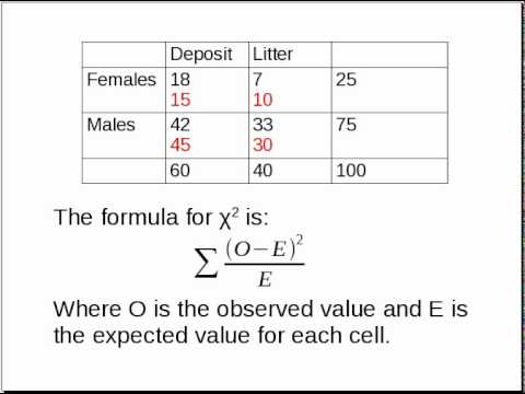
The chi-square statistic is computed using the formula:
\[
\chi^2 = \sum \frac{(O_i - E_i)^2}{E_i}
\]
Where \(O_i\) are the observed frequencies and \(E_i\) are the expected frequencies.
Calculating for each category:
- Category A: \(\frac{(50 - 40)^2}{40} = 2.5\)
- Category B: \(\frac{(30 - 30)^2}{30} = 0\)
- Category C: \(\frac{(15 - 20)^2}{20} = 1.25\)
- Category D: \(\frac{(5 - 10)^2}{10} = 2.5\)
Total chi-square statistic:
\[
\chi^2 = 2.5 + 0 + 1.25 + 2.5 = 6.25
\]
Degrees of Freedom
The degrees of freedom (df) are calculated as:
\[
\text{df} = \text{number of categories} - 1 = 4 - 1 = 3
\]
Conclusion
We compare the computed chi-square statistic (6.25) to the critical value from the chi-square distribution table at a specific significance level (e.g., 0.05) for 3 degrees of freedom. If the chi-square statistic is greater than the critical value, we reject the null hypothesis. Otherwise, we fail to reject the null hypothesis.
In this example, let's assume the critical value at 0.05 significance level for 3 degrees of freedom is 7.815. Since 6.25 < 7.815, we fail to reject the null hypothesis, meaning the observed frequencies fit the expected distribution.
READ MORE:
Introduction to Chi-Square Goodness of Fit Test
The Chi-Square Goodness of Fit Test is a non-parametric statistical test used to determine if a sample data set matches a population with a specific distribution. It helps assess how well the observed data fits the expected distribution. This test is particularly useful for categorical data and is widely applied in various fields such as biology, marketing, and social sciences.
Here are the key steps involved in performing the Chi-Square Goodness of Fit Test:
- Define the Hypotheses:
- Null Hypothesis (\(H_0\)): The observed frequencies match the expected frequencies.
- Alternative Hypothesis (\(H_a\)): The observed frequencies do not match the expected frequencies.
- Calculate the Expected Frequencies: The expected frequencies are determined based on the hypothesized distribution. For example, if we expect an equal distribution across four categories, the expected frequency for each category would be \( \frac{\text{Total Observations}}{4} \).
- Compute the Chi-Square Statistic: The chi-square statistic is calculated using the formula:
\[
\chi^2 = \sum \frac{(O_i - E_i)^2}{E_i}
\]Where \(O_i\) represents the observed frequencies and \(E_i\) represents the expected frequencies.
- Determine the Degrees of Freedom: The degrees of freedom (df) for the test are calculated as the number of categories minus one:
\[
\text{df} = \text{number of categories} - 1
\] - Compare the Computed Chi-Square Statistic to the Critical Value: Using the chi-square distribution table, find the critical value for the desired significance level (e.g., 0.05) and the calculated degrees of freedom. If the computed chi-square statistic exceeds the critical value, reject the null hypothesis.
The Chi-Square Goodness of Fit Test provides a robust method for evaluating the fit between observed data and expected distributions, making it an essential tool in statistical analysis.
Understanding the Null and Alternative Hypotheses
In the Chi-Square Goodness of Fit Test, the null and alternative hypotheses play a crucial role in determining whether the observed data matches the expected distribution. Here is a detailed explanation of each:
Null Hypothesis (\(H_0\))
The null hypothesis (\(H_0\)) is a statement that there is no significant difference between the observed frequencies and the expected frequencies. In other words, it suggests that any deviations are due to random chance. The null hypothesis can be expressed as:
\[
H_0: O_i = E_i \quad \text{for all categories}
\]
Where \(O_i\) represents the observed frequencies and \(E_i\) represents the expected frequencies.
Alternative Hypothesis (\(H_a\))
The alternative hypothesis (\(H_a\)) is a statement that there is a significant difference between the observed frequencies and the expected frequencies. This means that the observed data does not fit the expected distribution. The alternative hypothesis can be expressed as:
\[
H_a: O_i \neq E_i \quad \text{for at least one category}
\]
Formulating the Hypotheses
When performing the Chi-Square Goodness of Fit Test, it is essential to clearly define both hypotheses. Here is a step-by-step approach:
- Identify the Distribution: Determine the expected distribution for the data. This could be a uniform distribution, a specific proportion, or another theoretical distribution.
- Calculate Expected Frequencies: Based on the expected distribution, calculate the expected frequencies for each category. For example, if we expect a uniform distribution across four categories with 100 observations, the expected frequency for each category would be 25.
- State the Null Hypothesis: Formulate the null hypothesis stating that the observed frequencies match the expected frequencies.
- State the Alternative Hypothesis: Formulate the alternative hypothesis stating that the observed frequencies do not match the expected frequencies.
The Chi-Square Goodness of Fit Test then uses these hypotheses to determine if the observed data significantly deviates from the expected distribution. By comparing the calculated chi-square statistic to the critical value from the chi-square distribution table, we can decide whether to accept or reject the null hypothesis.
Calculating Expected Frequencies
Calculating the expected frequencies is a crucial step in performing the Chi-Square Goodness of Fit Test. The expected frequencies are derived from the hypothesized distribution and provide a basis for comparison with the observed frequencies. Here is a detailed, step-by-step process for calculating the expected frequencies:
- Determine the Total Number of Observations:
Calculate the total number of observations in the dataset. This is done by summing up all the observed frequencies.
For example, if we have the following observed frequencies for four categories:
- Category A: 50
- Category B: 30
- Category C: 15
- Category D: 5
The total number of observations (\(N\)) is:
\[
N = 50 + 30 + 15 + 5 = 100
\] - Identify the Hypothesized Distribution:
Determine the expected distribution for the categories. This could be an equal distribution, a specific proportion, or another theoretical distribution.
For example, if we expect the following distribution for the four categories:
- Category A: 40%
- Category B: 30%
- Category C: 20%
- Category D: 10%
- Calculate the Expected Frequencies:
Use the total number of observations and the hypothesized distribution to calculate the expected frequencies for each category. The expected frequency (\(E_i\)) for each category is calculated using the formula:
\[
E_i = p_i \times N
\]Where \(p_i\) is the proportion of the hypothesized distribution for category \(i\) and \(N\) is the total number of observations.
Applying this formula to our example:
- Category A: \(0.40 \times 100 = 40\)
- Category B: \(0.30 \times 100 = 30\)
- Category C: \(0.20 \times 100 = 20\)
- Category D: \(0.10 \times 100 = 10\)
The calculated expected frequencies are then used in the chi-square formula to compare against the observed frequencies. This comparison helps determine whether the observed data significantly deviates from the expected distribution, guiding the decision to accept or reject the null hypothesis.
Computing the Chi-Square Statistic
The chi-square statistic (\(\chi^2\)) is a measure used in statistical tests to determine the goodness of fit between observed and expected frequencies. Here are the detailed steps to compute the chi-square statistic:
-
Collect the Observed Frequencies: Begin by collecting the observed frequencies (\(O_i\)) for each category. These are the actual counts obtained from your data.
-
Calculate the Expected Frequencies: Calculate the expected frequencies (\(E_i\)) for each category. The expected frequency is determined under the null hypothesis and represents the theoretical frequency for each category if the null hypothesis is true. The formula for the expected frequency is:
\[ E_i = N \times P_i \]
where \(N\) is the total number of observations and \(P_i\) is the probability of the category under the null hypothesis.
-
Compute the Chi-Square Statistic: Use the observed and expected frequencies to compute the chi-square statistic using the formula:
\[ \chi^2 = \sum \frac{(O_i - E_i)^2}{E_i} \]
where \(O_i\) is the observed frequency and \(E_i\) is the expected frequency for category \(i\). This formula calculates the sum of the squared differences between observed and expected frequencies, divided by the expected frequency for each category.
Here is an example to illustrate the computation:
| Category | Observed Frequency (Oi) | Expected Frequency (Ei) | (Oi - Ei) | (Oi - Ei)^2 | \((O_i - E_i)^2 / E_i\) |
|---|---|---|---|---|---|
| Category 1 | 50 | 60 | -10 | 100 | 1.67 |
| Category 2 | 30 | 25 | 5 | 25 | 1.00 |
| Category 3 | 20 | 15 | 5 | 25 | 1.67 |
The chi-square statistic is calculated by summing the last column:
\[ \chi^2 = 1.67 + 1.00 + 1.67 = 4.34 \]
This computed chi-square statistic is then compared to a critical value from the chi-square distribution table, with the appropriate degrees of freedom, to determine the significance of the result. The degrees of freedom are calculated as:
\[ \text{Degrees of Freedom} = \text{Number of Categories} - 1 \]
If the chi-square statistic exceeds the critical value, the null hypothesis is rejected.
Determining Degrees of Freedom
In the context of a Chi-Square Goodness of Fit test, the degrees of freedom (df) play a crucial role in interpreting the test results. The degrees of freedom are determined based on the number of categories or levels in your data set.
To compute the degrees of freedom for a Chi-Square Goodness of Fit test, use the following formula:
$$df = k - 1$$
Where:
kis the number of categories or levels.
For example, if you are testing whether the distribution of colors in a bag of candy matches a specified distribution and there are 5 different colors, the degrees of freedom would be:
$$df = 5 - 1 = 4$$
Step-by-Step Example
Let's consider an example where we have a sample of candies in 5 different colors: red, green, blue, yellow, and purple. We want to determine if the observed frequencies match the expected frequencies based on a specified distribution.
- Count the number of categories: In this case, we have 5 colors.
- Apply the formula:
$$df = 5 - 1 = 4$$
Thus, the degrees of freedom for this test would be 4. These degrees of freedom are then used to find the critical value from the Chi-Square distribution table, which will help in deciding whether to reject the null hypothesis.
Why Degrees of Freedom Matter
The degrees of freedom are essential because they affect the shape of the Chi-Square distribution. Higher degrees of freedom result in a distribution that is more spread out. When performing the Chi-Square test, we compare the calculated Chi-Square statistic to a critical value from the Chi-Square distribution table with the corresponding degrees of freedom and significance level (often 0.05).
For instance, with 4 degrees of freedom and a significance level of 0.05, the critical value is approximately 9.488. If your Chi-Square statistic is greater than this critical value, you reject the null hypothesis, indicating that there is a significant difference between the observed and expected frequencies.
In summary, determining the degrees of freedom is a straightforward yet critical step in performing a Chi-Square Goodness of Fit test, as it directly influences the test's outcome and the conclusions you can draw from your data.
Interpreting the Chi-Square Test Results
Once you have computed the Chi-Square statistic, the next step is to interpret the results to determine whether to reject the null hypothesis. The following steps outline the process:
-
Determine the Degrees of Freedom (df):
For the Chi-Square Goodness of Fit Test, the degrees of freedom are calculated as:
where n is the number of categories.
-
Find the Critical Value:
Using a Chi-Square distribution table, find the critical value based on the calculated degrees of freedom and the chosen significance level (α, commonly 0.05).
Degrees of Freedom (df) Significance Level (α = 0.05) 1 3.841 2 5.991 3 7.815 4 9.488 -
Compare the Chi-Square Statistic to the Critical Value:
If the calculated Chi-Square statistic is greater than the critical value from the table, you reject the null hypothesis.
-
Draw a Conclusion:
Based on the comparison, interpret the results:
- Reject the null hypothesis: If the Chi-Square statistic is greater than the critical value, there is sufficient evidence to conclude that the observed frequencies significantly differ from the expected frequencies.
- Fail to reject the null hypothesis: If the Chi-Square statistic is less than or equal to the critical value, there is not enough evidence to conclude that the observed frequencies significantly differ from the expected frequencies.
Example:
Suppose you have the following observed and expected frequencies for a survey of favorite colors among 100 people:
| Color | Observed (O) | Expected (E) |
|---|---|---|
| Red | 30 | 25 |
| Blue | 40 | 25 |
| Green | 20 | 25 |
| Yellow | 10 | 25 |
Calculate the Chi-Square statistic:
Degrees of Freedom:
Using a significance level of 0.05, the critical value from the table is 7.815. Compare this value to your calculated Chi-Square statistic to draw your conclusion.
By following these steps, you can effectively interpret the results of your Chi-Square Goodness of Fit Test and determine the validity of your null hypothesis.
Step-by-Step Example of Chi-Square Goodness of Fit Test
Let's walk through a detailed example of performing a Chi-Square Goodness of Fit test. We'll use a scenario involving a package of M&Ms to determine if the colors are distributed equally.
Step 1: State the Hypotheses
- Null Hypothesis (\(H_0\)): The colors are distributed equally. Each color has an expected proportion of \( \frac{1}{6} \).
- Alternative Hypothesis (\(H_a\)): At least one color has a different proportion.
Step 2: Collect and Summarize the Data
Suppose we have a sample of 600 M&Ms with the following observed counts:
| Color | Observed Count | Expected Count |
|---|---|---|
| Blue | 212 | 100 |
| Orange | 147 | 100 |
| Green | 103 | 100 |
| Red | 50 | 100 |
| Yellow | 46 | 100 |
| Brown | 42 | 100 |
Step 3: Calculate the Chi-Square Statistic
We use the formula:
\[
\chi^2 = \sum \frac{(O_i - E_i)^2}{E_i}
\]
where \( O_i \) is the observed frequency and \( E_i \) is the expected frequency.
Calculating each term:
- Blue: \(\frac{(212 - 100)^2}{100} = 125.44\)
- Orange: \(\frac{(147 - 100)^2}{100} = 22.09\)
- Green: \(\frac{(103 - 100)^2}{100} = 0.09\)
- Red: \(\frac{(50 - 100)^2}{100} = 25.00\)
- Yellow: \(\frac{(46 - 100)^2}{100} = 29.16\)
- Brown: \(\frac{(42 - 100)^2}{100} = 33.64\)
Summing these values gives the Chi-Square statistic:
\[
\chi^2 = 125.44 + 22.09 + 0.09 + 25.00 + 29.16 + 33.64 = 235.42
\]
Step 4: Determine the Degrees of Freedom
The degrees of freedom (df) is calculated as:
\[
df = k - 1
\]
where \( k \) is the number of categories. For our example, \( k = 6 \), so:
\[
df = 6 - 1 = 5
\]
Step 5: Find the P-Value
Using a Chi-Square distribution table or calculator, we find the p-value for \(\chi^2 = 235.42\) with 5 degrees of freedom. The p-value is extremely small (almost zero), indicating strong evidence against the null hypothesis.
Step 6: Make a Decision
Since the p-value is less than the significance level (usually 0.05), we reject the null hypothesis. This suggests that the colors are not equally distributed in the M&Ms package.
Using Chi-Square Distribution Table
The chi-square distribution table is an essential tool for interpreting the results of a chi-square test. Here's a detailed, step-by-step guide on how to use this table effectively:
-
Calculate the Chi-Square Statistic:
The chi-square statistic is computed using the formula:
\[
\chi^2 = \sum \frac{(O - E)^2}{E}
\]
where \( O \) represents the observed frequency, and \( E \) represents the expected frequency. -
Determine the Degrees of Freedom (df):
The degrees of freedom for the chi-square goodness-of-fit test are calculated as:
\[
\text{df} = k - 1
\]
where \( k \) is the number of categories or possible outcomes. -
Select the Significance Level (α):
Common significance levels are 0.05, 0.01, and 0.10. This value represents the probability of rejecting the null hypothesis when it is actually true.
-
Find the Critical Value:
Using the chi-square distribution table, locate the critical value that corresponds to your chosen significance level (α) and the degrees of freedom (df). The table provides critical values for different levels of significance and degrees of freedom.
-
Compare the Chi-Square Statistic to the Critical Value:
If the calculated chi-square statistic is greater than the critical value from the table, you reject the null hypothesis. This indicates that there is a significant difference between the observed and expected frequencies.
-
For example, if your chi-square statistic is 10.5, your degrees of freedom are 4, and your significance level is 0.05, you would find the critical value for 4 degrees of freedom and α = 0.05 in the table. If the critical value is 9.488, since 10.5 > 9.488, you reject the null hypothesis.
-
Here's an example chi-square distribution table for selected degrees of freedom and significance levels:
| Degrees of Freedom (df) | 0.10 | 0.05 | 0.01 |
|---|---|---|---|
| 1 | 2.706 | 3.841 | 6.635 |
| 2 | 4.605 | 5.991 | 9.210 |
| 3 | 6.251 | 7.815 | 11.345 |
| 4 | 7.779 | 9.488 | 13.277 |
Using the chi-square distribution table allows you to determine whether your observed data significantly deviates from the expected distribution. This helps in making informed decisions based on statistical evidence.

Assumptions and Limitations of Chi-Square Goodness of Fit Test
The Chi-Square Goodness of Fit test is a powerful tool for determining if observed categorical data matches an expected distribution. However, there are several key assumptions and limitations to consider when using this test:
Assumptions
- Random Sampling: The data must be collected through a process of random sampling to ensure that the sample accurately represents the population.
- Independence: Each observation must be independent of all others. This means that the occurrence of one event does not affect the occurrence of another.
- Expected Frequency: Each category should have an expected frequency of at least 5. This ensures the reliability of the test statistics.
- Categorical Data: The variables being tested must be categorical. Chi-square tests are not suitable for continuous data.
Limitations
- Sensitivity to Sample Size: The Chi-Square test is sensitive to the size of the sample. Very large samples can result in statistically significant results even for small deviations from the expected distribution, while very small samples may not have enough power to detect a real difference.
- Frequency Data Requirement: The test requires frequency data, meaning that the data must be in the form of counts of occurrences in each category.
- Non-Negative Data: All observed and expected frequencies must be non-negative. Negative values are not permissible in Chi-Square calculations.
- Not Informative About Magnitude: The Chi-Square test indicates whether there is a significant difference but does not provide information about the magnitude of the difference.
- Cannot Handle Zero Frequencies: If any of the expected frequencies are zero, the Chi-Square test cannot be used directly. This might require combining categories or using an alternative test.
Understanding these assumptions and limitations is crucial for properly applying the Chi-Square Goodness of Fit test and correctly interpreting its results.
Applications of Chi-Square Goodness of Fit Test in Real-World Scenarios
The Chi-Square Goodness of Fit Test is widely used in various fields to determine if observed data fits a specified distribution. Below are several real-world applications:
1. Retail and Customer Behavior
Retailers often use the Chi-Square Goodness of Fit Test to analyze customer behavior patterns. For instance:
- Counting Customers: A shop owner may want to know if an equal number of customers visit the store each day of the week. By counting the number of customers daily and using the Chi-Square test, the owner can determine if the observed distribution deviates significantly from the expected equal distribution.
2. Quality Control in Manufacturing
In manufacturing, ensuring product quality and consistency is crucial. The Chi-Square test helps in validating this:
- Testing Product Defects: Manufacturers can test if the number of defective products across different batches follows a uniform distribution, which helps in identifying any irregularities in the production process.
3. Medical Research
Medical researchers use the Chi-Square Goodness of Fit Test to verify theoretical distributions in their studies:
- Genetic Studies: Researchers may want to determine if the distribution of certain genetic traits in a population fits the expected Mendelian inheritance patterns.
4. Marketing and Advertising
In marketing, understanding consumer preferences is key to effective advertising strategies:
- Consumer Preferences: Marketers might use the test to see if the observed frequencies of consumer preferences for different product categories fit the expected market distribution, aiding in targeted advertising campaigns.
5. Environmental Studies
Environmental scientists apply the Chi-Square test to ecological data:
- Species Distribution: Ecologists may test if the observed distribution of a species in different habitats conforms to a hypothesized distribution, helping in conservation efforts.
6. Education and Psychology
In education and psychology, researchers use the Chi-Square test to analyze categorical data:
- Survey Analysis: Psychologists may use the test to determine if responses to a survey question follow the expected distribution based on a theoretical model of behavior.
7. Fairness of Random Devices
Testing the fairness of random devices is a common application:
- Testing if a Die is Fair: A researcher can roll a die multiple times and use the Chi-Square test to check if the outcomes follow a uniform distribution, indicating whether the die is fair.
These applications demonstrate the versatility of the Chi-Square Goodness of Fit Test in various domains, providing valuable insights and helping in decision-making processes.
Common Mistakes and How to Avoid Them
The Chi-Square Goodness of Fit Test is a powerful tool, but there are several common mistakes that can lead to incorrect conclusions. Here are some of these mistakes and how to avoid them:
- Using Inappropriate Data:
The chi-square test is designed for categorical data. Using continuous data can lead to misleading results. Always ensure your data is categorical.
- Expected Frequencies Too Low:
If expected frequencies are too low (less than 5 in any cell), the chi-square test may not be valid. Consider combining categories or using a different statistical test if this occurs.
- Incorrect Degrees of Freedom:
Ensure you calculate the degrees of freedom correctly as , where is the number of categories. Incorrect degrees of freedom can lead to wrong critical value selection and p-value calculation.
- Misinterpreting the P-Value:
The p-value indicates the probability that the observed data would occur if the null hypothesis were true. A common mistake is to interpret a high p-value as proof that the null hypothesis is true. Instead, it means there is insufficient evidence to reject the null hypothesis.
- Not Checking Assumptions:
The chi-square test assumes that the observations are independent and the sample size is sufficiently large. Violating these assumptions can invalidate the test results. Always check these assumptions before applying the test.
- Incorrect Calculation of Expected Frequencies:
Expected frequencies should be calculated based on the null hypothesis. Errors in this step can significantly affect the test outcome. Double-check your calculations to ensure accuracy.
By being aware of these common mistakes and taking steps to avoid them, you can ensure the validity and reliability of your chi-square goodness of fit test results.
Chi-Square Goodness of Fit Test in Different Software
The Chi-Square Goodness of Fit Test can be performed using various statistical software packages. Below are detailed steps on how to conduct this test using some of the most commonly used software: Excel, SPSS, R, and Python.
Using Excel
- Input your observed and expected frequencies in two columns.
- Calculate the Chi-Square statistic using the formula:
where \(O_i\) is the observed frequency and \(E_i\) is the expected frequency.
\[
\chi^2 = \sum \frac{(O_i - E_i)^2}{E_i}
\] - Use the Excel function
=CHISQ.TEST(actual_range, expected_range)to get the p-value. - Compare the p-value with your significance level to make a decision.
Using SPSS
- Enter your data in the Data View.
- Navigate to Analyze > Nonparametric Tests > Legacy Dialogs > Chi-Square.
- Select the variable you want to test and specify the expected values.
- Run the test and interpret the output, focusing on the Chi-Square statistic and p-value.
Using R
- Install the necessary package if not already installed:
install.packages("stats"). - Use the following code to perform the test:
observed <- c(180, 250, 120, 225, 225) expected <- c(200, 200, 200, 200, 200) chisq.test(observed, p = expected/sum(expected)) - Review the output to find the Chi-Square statistic and p-value.
Using Python
- Install the
scipylibrary if not already installed:pip install scipy. - Use the following code to perform the test:
from scipy.stats import chisquare observed = [180, 250, 120, 225, 225] expected = [200, 200, 200, 200, 200] chisquare(observed, expected) - Interpret the result, focusing on the Chi-Square statistic and p-value.
Each software provides a slightly different interface and method for performing the Chi-Square Goodness of Fit Test, but they all fundamentally rely on comparing the observed frequencies to the expected frequencies and determining the significance of the differences.
Chi-Square Test vs. Other Statistical Tests
When comparing the Chi-Square goodness of fit test with other statistical tests, it's essential to understand the distinct scenarios where each test is applicable:
- Chi-Square Test: Primarily used to determine if there is a significant difference between the observed and expected frequencies of categorical data. It's robust for non-normal distributions and involves comparing frequencies rather than means.
- Student's t-test: Used to determine if there is a significant difference between the means of two groups. It assumes the data follows a normal distribution and is sensitive to outliers.
- ANOVA (Analysis of Variance): Suitable for comparing means across multiple groups simultaneously. ANOVA tests whether there are any statistically significant differences between the means of three or more independent groups.
- Z-test: Used for testing the mean of a distribution against a known value, or to compare two means when the population standard deviation is known.
Choosing the right test depends on the nature of the data and the specific hypotheses being tested. While Chi-Square tests are powerful for categorical data, tests like t-tests and ANOVA are more appropriate for continuous data that approximate a normal distribution.
Advanced Topics in Chi-Square Goodness of Fit Test
- Effect Size Measures: Understanding measures like Cramer's V or Phi coefficient to assess the strength of association in Chi-Square tests.
- Post-Hoc Analysis: Techniques for exploring significant results further, such as residual analysis or pairwise comparisons.
- Simulation Studies: Using Monte Carlo simulations to evaluate the performance of Chi-Square tests under various conditions.
- Adjusted Residuals: Utilizing adjusted residuals to identify which categories contribute most to significant Chi-Square results.
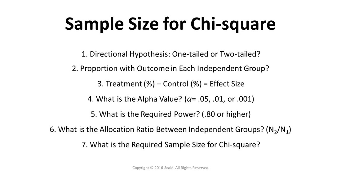
- Power Analysis: Assessing the statistical power of Chi-Square tests to detect a significant difference, based on sample size and expected effect size.
FAQs on Chi-Square Goodness of Fit Test
- What is a Chi-Square Goodness of Fit Test?
A Chi-Square goodness of fit test assesses whether the observed categorical data fits a theoretical distribution.
- When should I use a Chi-Square Goodness of Fit Test?
Use it when you have categorical data and want to test whether the observed frequencies match the expected frequencies.
- How do you interpret the Chi-Square statistic?
A larger Chi-Square statistic indicates a greater discrepancy between observed and expected frequencies, suggesting a less likely fit to the theoretical distribution.
- What are the assumptions of a Chi-Square Goodness of Fit Test?
Assumptions include independence of observations, and expected frequencies should not be too small (typically greater than 5).
- What if my expected frequencies are not met?
You may need to combine categories or choose an alternative test method depending on the specific situation and data distribution.
Xem video về Kiểm Định Chi-Square của Pearson để hiểu về phân phối và thống kê trong xác suất.
Video Kiểm Định Chi-Square của Pearson | Xác suất và Thống kê | Khan Academy
READ MORE:
Xem video về Kiểm Định Chi-Square để hiểu cách áp dụng và phân tích kết quả một cách chi tiết.
Video Kiểm Định Chi-Square cho Sự Phù Hợp

:max_bytes(150000):strip_icc()/Chi-SquareStatistic_Final_4199464-7eebcd71a4bf4d9ca1a88d278845e674.jpg)