Topic chi square test of independence example: The chi-square test of independence is a statistical method used to determine if there is a significant association between two categorical variables. This guide provides a clear example, step-by-step instructions, and practical applications to help you understand and perform the test effectively.
Table of Content
- Chi-Square Test of Independence Example
- Introduction
- What is a Chi-Square Test of Independence?
- When to Use the Chi-Square Test of Independence
- Assumptions and Requirements
- Steps to Perform a Chi-Square Test of Independence
- Example: Gender and Political Party Preference
- Example: Movie Type and Snack Purchases
- Calculating the Test Statistic
- Interpreting the Results
- Conclusion
- YOUTUBE:
Chi-Square Test of Independence Example
The Chi-Square Test of Independence is used to determine if there is a significant association between two categorical variables. This test is commonly applied in scenarios like election surveys, where voters are classified by gender and voting preference.
Example Scenario
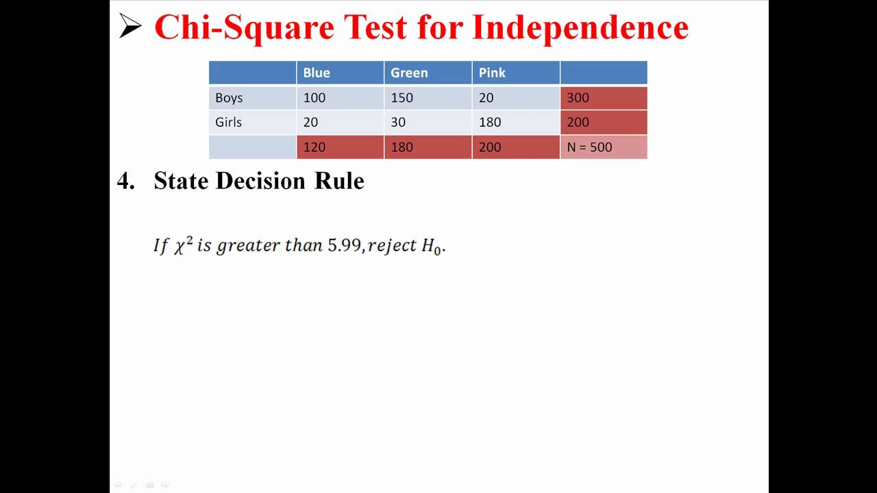
Consider a survey of 500 voters classified by gender (Male, Female) and political party preference (Republican, Democrat, Independent). The observed data is:
| Republican | Democrat | Independent | Total | |
| Male | 120 | 90 | 40 | 250 |
| Female | 110 | 95 | 45 | 250 |
| Total | 230 | 185 | 85 | 500 |
Steps to Perform Chi-Square Test of Independence
Step 1: Define the Hypotheses
- Null Hypothesis (H0): Gender and political party preference are independent.
- Alternative Hypothesis (H1): Gender and political party preference are not independent.
Step 2: Calculate the Expected Values
The expected value for each cell is calculated using the formula:
\( \text{Expected value} = \frac{\text{row sum} \times \text{column sum}}{\text{total sum}} \)
For example, the expected value for Male Republicans is:
\( \text{Expected value} = \frac{230 \times 250}{500} = 115 \)
| Republican | Democrat | Independent | Total | |
| Male | 115 | 92.5 | 42.5 | 250 |
| Female | 115 | 92.5 | 42.5 | 250 |
| Total | 230 | 185 | 85 | 500 |
Step 3: Calculate Chi-Square Statistic
Calculate \( \frac{(O - E)^2}{E} \) for each cell:
For Male Republicans:
\( \frac{(120 - 115)^2}{115} = 0.2174 \)
Repeat for all cells to get the Chi-Square statistic:
\( \chi^2 = \sum \frac{(O - E)^2}{E} = 0.2174 + 0.2174 + 0.0676 + 0.0676 + 0.1471 + 0.1471 = 0.8642 \)
Step 4: Determine the p-value and Conclusion
The p-value is calculated based on the Chi-Square statistic and degrees of freedom:
Degrees of freedom (df) = (number of rows - 1) * (number of columns - 1) = (2-1) * (3-1) = 2
Using a Chi-Square distribution table or calculator, we find the p-value associated with \( \chi^2 = 0.8642 \) and df = 2. Let's say it is 0.6492.
Since the p-value (0.6492) is greater than the significance level (0.05), we fail to reject the null hypothesis. Thus, we do not have sufficient evidence to say there is an association between gender and political party preference.
Additional Resources
- How to Perform a Chi-Square Test of Independence in R
- Chi-Square Test of Independence Calculator
- How to Calculate the P-Value of a Chi-Square Statistic in R

READ MORE:
Introduction
The Chi-Square Test of Independence is a statistical method used to determine if there is a significant association between two categorical variables. This test compares the observed frequencies in each category of a contingency table to the frequencies that would be expected if the variables were independent. By calculating the chi-square statistic and comparing it to a critical value from the chi-square distribution, researchers can assess whether any observed deviations from independence are statistically significant.
To perform a Chi-Square Test of Independence, follow these steps:
- Formulate the hypotheses:
- Null hypothesis (H0): The two variables are independent.
- Alternative hypothesis (H1): The two variables are not independent.
- Construct a contingency table and calculate the expected frequencies for each cell using the formula: \[ \text{Expected frequency} = \frac{\text{Row total} \times \text{Column total}}{\text{Grand total}} \]
- Calculate the chi-square statistic using the formula: \[ \chi^2 = \sum \frac{(O - E)^2}{E} \] where \(O\) is the observed frequency and \(E\) is the expected frequency.
- Determine the degrees of freedom (df) for the test, which is given by: \[ \text{df} = (\text{number of rows} - 1) \times (\text{number of columns} - 1) \]
- Compare the calculated chi-square statistic to the critical value from the chi-square distribution table at the chosen significance level (commonly 0.05). If the chi-square statistic exceeds the critical value, reject the null hypothesis.
The Chi-Square Test of Independence is widely used in various fields, including social sciences, biology, and marketing, to explore the relationships between categorical variables. It is a powerful tool for understanding data patterns and making data-driven decisions.
What is a Chi-Square Test of Independence?
The Chi-Square Test of Independence is a statistical test used to determine if there is a significant association between two categorical variables. It is widely used in research to assess whether observed frequencies differ from expected frequencies under the assumption of no association. The test compares the observed data with the data we would expect to obtain according to a specific hypothesis.
To perform a Chi-Square Test of Independence, follow these steps:
-
Set up your hypotheses:
- Null hypothesis (H0): Assumes there is no association between the two variables.
- Alternative hypothesis (H1): Assumes there is an association between the two variables.
-
Create a contingency table:
Organize the data into a table showing the frequency distribution of the variables. Each cell represents the frequency count of occurrences for specific combinations of the variables.
-
Calculate the expected frequencies:
Use the formula: \( e_{ij} = \frac{(o_i \cdot o_j)}{N} \)
Where:
- \( e_{ij} \) = expected frequency for cell (i,j)
- \( o_i \) = total frequency for row i
- \( o_j \) = total frequency for column j
- \( N \) = total sample size
-
Compute the Chi-Square statistic:
Use the formula: \( \chi^2 = \sum \frac{(o_{ij} - e_{ij})^2}{e_{ij}} \)
Where:
- \( \chi^2 \) = Chi-Square statistic
- \( o_{ij} \) = observed frequency for cell (i,j)
- \( e_{ij} \) = expected frequency for cell (i,j)
-
Determine the degrees of freedom:
Use the formula: \( df = (r-1) \cdot (c-1) \)
Where:
- \( r \) = number of rows
- \( c \) = number of columns
-
Compare the Chi-Square statistic to the critical value:
Using a Chi-Square distribution table, find the critical value for your calculated degrees of freedom and chosen significance level (e.g., 0.05). If the Chi-Square statistic is greater than the critical value, reject the null hypothesis.
The Chi-Square Test of Independence provides valuable insights into the relationships between categorical variables and is an essential tool in various fields such as social sciences, marketing, and medical research.
When to Use the Chi-Square Test of Independence
The Chi-Square Test of Independence is a statistical method used to determine if there is a significant association between two categorical variables. It is particularly useful in the following scenarios:
- Comparing Proportions: When you want to compare the proportions of categories across different groups. For instance, examining if there is a relationship between gender (male/female) and voting preference (party A/party B).
- Two Categorical Variables: When your data involves two categorical variables and you want to see if they are independent of each other. Examples include the relationship between educational level (high school, undergraduate, graduate) and employment status (employed, unemployed).
- Survey Data Analysis: When analyzing survey data to find associations between different questions that have categorical responses. For instance, determining if customer satisfaction (satisfied, not satisfied) is related to the type of service received (online, in-person).
- Experimental Research: In experimental research, when you need to test the relationship between different categorical factors. For example, testing if different teaching methods (lecture, interactive) influence the pass rate (pass, fail) among students.
- Independence Testing: To test the independence of variables such as in genetics to see if two traits are inherited independently.
Before using the Chi-Square Test of Independence, ensure the following conditions are met:
- Independence of Observations: The data should consist of independent observations. Each subject or entity should only be counted once in the dataset.
- Expected Frequency: The expected frequency in each cell of the contingency table should be at least 5 for the Chi-Square approximation to be valid.
Assumptions and Requirements
The Chi-Square Test of Independence is used to determine whether there is a significant association between two categorical variables. To ensure the validity of the test, several key assumptions and requirements must be met:
- Both variables are categorical. This means that the variables can take on names or labels rather than numerical values. Examples include marital status (e.g., married, single) and political preference (e.g., republican, democrat).
- All observations are independent. Each observation in the dataset must be independent of every other observation. This is typically ensured by using a proper random sampling method.
- The cells in the contingency table are mutually exclusive. Each individual or observation can only belong to one cell in the table, meaning that categories are distinct and do not overlap.
- The expected frequency count in each cell of the table should be at least 5 in at least 80% of the cells. Additionally, no cell should have an expected frequency of less than 1.
By meeting these assumptions, the results of the Chi-Square Test of Independence will be more reliable and accurate.
Steps to Perform a Chi-Square Test of Independence
To perform a Chi-Square Test of Independence, follow these detailed steps:
-
Calculate the Totals: Sum each row and column in your contingency table to find the row totals, column totals, and the overall total.
Group A Group B Total Category 1 Observed Value 1 Observed Value 2 Row Total 1 Category 2 Observed Value 3 Observed Value 4 Row Total 2 Total Column Total 1 Column Total 2 Overall Total -
Calculate Expected Values: For each cell in the table, calculate the expected value using the formula:
\[ \text{Expected Value} = \frac{\text{(Row Total)} \times \text{(Column Total)}}{\text{Overall Total}} \]
-
Compute Chi-Square Statistic: For each cell, calculate the chi-square statistic using:
\[ \chi^2 = \sum \frac{(\text{Observed Value} - \text{Expected Value})^2}{\text{Expected Value}} \]
-
Determine Degrees of Freedom: The degrees of freedom (df) is calculated by:
\[ df = (r - 1) \times (c - 1) \]
where \( r \) is the number of rows and \( c \) is the number of columns.
-
Find the P-Value: Use the chi-square statistic and degrees of freedom to find the p-value from the chi-square distribution.
-
Interpret Results: Compare the p-value to your significance level (\(\alpha\)). If the p-value is less than \(\alpha\), reject the null hypothesis, indicating a significant association between the variables.
Example: Gender and Political Party Preference
To illustrate the Chi-Square Test of Independence, let's consider an example examining the relationship between gender and political party preference. The data is collected from a sample of 500 individuals who were asked about their gender and political party preference. The observed frequencies are as follows:
| Republican | Democrat | Independent | Total | |
| Male | 120 | 90 | 40 | 250 |
| Female | 110 | 95 | 45 | 250 |
| Total | 230 | 185 | 85 | 500 |
To perform the Chi-Square Test of Independence, we follow these steps:
- Define the null and alternative hypotheses:
- Null hypothesis (\(H_0\)): Gender and political party preference are independent.
- Alternative hypothesis (\(H_1\)): Gender and political party preference are not independent.
- Calculate the expected frequencies for each cell using the formula:
\[ E_{ij} = \frac{(Row\ Total \times Column\ Total)}{Total\ Number\ of\ Observations} \] - Compute the expected values for each cell:
Republican Democrat Independent Male 115 92.5 42.5 Female 115 92.5 42.5 - Apply the Chi-Square formula:
\[ \chi^2 = \sum \frac{(O_{ij} - E_{ij})^2}{E_{ij}} \]
where \(O_{ij}\) is the observed frequency and \(E_{ij}\) is the expected frequency. - Calculate the Chi-Square statistic:
\[ \chi^2 = \frac{(120-115)^2}{115} + \frac{(90-92.5)^2}{92.5} + \frac{(40-42.5)^2}{42.5} + \frac{(110-115)^2}{115} + \frac{(95-92.5)^2}{92.5} + \frac{(45-42.5)^2}{42.5} \]
After calculation, the Chi-Square statistic is found to be approximately 0.866. - Determine the degrees of freedom (df):
\[ df = (number\ of\ rows - 1) \times (number\ of\ columns - 1) = (2-1) \times (3-1) = 2 \] - Compare the Chi-Square statistic to the critical value from the Chi-Square distribution table for \(df = 2\) at a significance level of 0.05, which is 5.991.
- Make a decision: Since 0.866 < 5.991, we fail to reject the null hypothesis. Thus, we do not have sufficient evidence to say that there is an association between gender and political party preference.
This example demonstrates how to use the Chi-Square Test of Independence to analyze categorical data and test for independence between two variables.
Example: Movie Type and Snack Purchases
In this example, we will examine if there is an association between the type of movie watched and the type of snack purchased at a movie theater. We will use a Chi-Square Test of Independence to analyze the data.
Consider the following observed data collected from a survey:
| Movie Type | Popcorn | Nachos | Candy | Soft Drinks | Total |
|---|---|---|---|---|---|
| Action | 40 | 25 | 30 | 50 | 145 |
| Comedy | 30 | 35 | 20 | 30 | 115 |
| Drama | 20 | 15 | 25 | 20 | 80 |
| Total | 90 | 75 | 75 | 100 | 340 |
To perform the Chi-Square Test of Independence, follow these steps:
- Calculate the expected frequencies for each cell in the table using the formula:
\( E_{ij} = \frac{(Row\ Total_i) \times (Column\ Total_j)}{Grand\ Total} \)
- Calculate the Chi-Square statistic using the formula:
\( \chi^2 = \sum \frac{(O_{ij} - E_{ij})^2}{E_{ij}} \)
- \( O_{ij} \) = observed frequency in cell (i, j)
- \( E_{ij} \) = expected frequency in cell (i, j)
- Determine the degrees of freedom (df):
\( df = (r - 1) \times (c - 1) \)
- r = number of rows
- c = number of columns
- Compare the calculated Chi-Square statistic to the critical value from the Chi-Square distribution table at the desired significance level (usually 0.05) with the appropriate degrees of freedom.
- Draw a conclusion:
- If the calculated Chi-Square statistic is greater than the critical value, reject the null hypothesis (there is an association between movie type and snack purchases).
- If the calculated Chi-Square statistic is less than or equal to the critical value, fail to reject the null hypothesis (there is no association between movie type and snack purchases).
Let's calculate the expected frequencies for the first cell (Action, Popcorn):
\( E_{11} = \frac{145 \times 90}{340} = 38.38 \)
Following similar calculations for all cells, we can populate the expected frequency table.
After calculating the expected frequencies and the Chi-Square statistic, we can interpret the results based on the steps outlined above.
Calculating the Test Statistic
The Chi-Square test statistic is calculated using the observed and expected frequencies from a contingency table. Here are the detailed steps to perform the calculation:
-
State the hypotheses:
- Null hypothesis (\(H_0\)): The two categorical variables are independent.
- Alternative hypothesis (\(H_1\)): The two categorical variables are not independent.
-
Construct the contingency table:
Let's consider an example where we study the relationship between movie type preference (Action, Comedy, Drama) and snack purchases (Popcorn, Candy, No Snack). We gather data and create the following observed frequency table:
Movie Type Popcorn Candy No Snack Total Action 30 10 10 50 Comedy 20 20 10 50 Drama 10 10 30 50 Total 60 40 50 150 -
Calculate the expected frequencies:
The expected frequency for each cell is calculated using the formula:
\[ E_{ij} = \frac{(row \, total \times column \, total)}{grand \, total} \]
For example, the expected frequency for the Action-Popcorn cell is:
\[ E_{11} = \frac{(50 \times 60)}{150} = 20 \]
Applying this formula, we get the following expected frequency table:
Movie Type Popcorn Candy No Snack Total Action 20 13.33 16.67 50 Comedy 20 13.33 16.67 50 Drama 20 13.33 16.67 50 Total 60 40 50 150 -
Compute the Chi-Square test statistic:
The test statistic is calculated using the formula:
\[ \chi^2 = \sum \frac{(O_{ij} - E_{ij})^2}{E_{ij}} \]
Where \(O_{ij}\) is the observed frequency and \(E_{ij}\) is the expected frequency. Let's calculate this for each cell:
- Action-Popcorn: \((30 - 20)^2 / 20 = 5\)
- Action-Candy: \((10 - 13.33)^2 / 13.33 = 0.832\)
- Action-No Snack: \((10 - 16.67)^2 / 16.67 = 2.668\)
- Comedy-Popcorn: \((20 - 20)^2 / 20 = 0\)
- Comedy-Candy: \((20 - 13.33)^2 / 13.33 = 3.34\)
- Comedy-No Snack: \((10 - 16.67)^2 / 16.67 = 2.668\)
- Drama-Popcorn: \((10 - 20)^2 / 20 = 5\)
- Drama-Candy: \((10 - 13.33)^2 / 13.33 = 0.832\)
- Drama-No Snack: \((30 - 16.67)^2 / 16.67 = 10.832\)
Summing these values gives us the test statistic:
\[ \chi^2 = 5 + 0.832 + 2.668 + 0 + 3.34 + 2.668 + 5 + 0.832 + 10.832 = 31.172 \]
-
Determine the degrees of freedom and the p-value:
The degrees of freedom for the test are calculated as:
\[ (r-1)(c-1) = (3-1)(3-1) = 4 \]
Using a Chi-Square distribution table or calculator, we find the p-value corresponding to the test statistic \(\chi^2 = 31.172\) with 4 degrees of freedom.
-
Make a decision:
If the p-value is less than the chosen significance level (e.g., 0.05), we reject the null hypothesis and conclude that there is a significant association between the movie type and snack purchases.
Interpreting the Results
After calculating the Chi-Square test statistic and obtaining the p-value, the next step is to interpret the results to make a conclusion about the independence of the variables. Here are the steps to interpret the results:
-
State the Hypotheses:
- Null Hypothesis (\(H_0\)): The two variables are independent.
- Alternative Hypothesis (\(H_1\)): The two variables are not independent.
-
Determine the Significance Level:
The significance level (\(\alpha\)) is typically set at 0.05. This represents the probability of rejecting the null hypothesis when it is actually true. It is the threshold for determining whether the observed association is statistically significant.
-
Compare the p-value to the Significance Level:
If the p-value is less than or equal to the significance level (\(\alpha\)), you reject the null hypothesis. This suggests that there is sufficient evidence to conclude that there is an association between the two variables.
If the p-value is greater than the significance level (\(\alpha\)), you fail to reject the null hypothesis. This suggests that there is not enough evidence to conclude that there is an association between the two variables.
-
Example Interpretation:
Assume we performed a Chi-Square test of independence on the relationship between movie type and snack purchases, and obtained the following results:
- Chi-Square test statistic (\( \chi^2 \)): 65.03
- Degrees of freedom (df): 3
- p-value: 0.001
Since the p-value (0.001) is less than the significance level (0.05), we reject the null hypothesis. Therefore, we conclude that there is a significant association between movie type and snack purchases.
-
Consider Practical Significance:
Statistical significance does not always imply practical significance. Consider the context and the magnitude of the association to determine if the result is meaningful in a real-world scenario.
In summary, interpreting the results of a Chi-Square test of independence involves comparing the p-value to the significance level to determine whether to reject the null hypothesis. If the null hypothesis is rejected, it indicates that there is a statistically significant association between the variables under study.
Conclusion
The Chi-Square Test of Independence is a powerful statistical tool used to determine if there is a significant association between two categorical variables. By following the steps of defining hypotheses, calculating expected values, computing the test statistic, and interpreting the results, researchers can draw meaningful conclusions about their data.
In the examples provided, we examined the relationship between movie type and snack purchases, and between gender and political party preference. Both examples illustrated the importance of calculating expected frequencies and the test statistic to determine the independence of variables.
When interpreting the results, it is crucial to compare the p-value with the significance level (usually 0.05). If the p-value is less than the significance level, we reject the null hypothesis, suggesting an association between the variables. If the p-value is greater, we fail to reject the null hypothesis, indicating insufficient evidence to support an association.
Ultimately, the Chi-Square Test of Independence helps in making data-driven decisions and understanding the relationships within categorical data. It is widely used in various fields, including social sciences, marketing, and health sciences, to analyze and interpret data effectively.
By mastering this statistical test, researchers can confidently explore and establish connections between categorical variables, enhancing their ability to make informed decisions based on empirical evidence.
Kiểm Tra Độc Lập Chi-Square
READ MORE:
Kiểm Tra Độc Lập Sử Dụng Phân Phối Chi-Square
:max_bytes(150000):strip_icc()/Chi-SquareStatistic_Final_4199464-7eebcd71a4bf4d9ca1a88d278845e674.jpg)