Topic chi square test sample size: Understanding the importance of sample size in chi-square tests is crucial for accurate statistical analysis. This guide delves into the key factors influencing sample size determination, offering practical tips and insights to help you achieve reliable and valid results in your research. Discover the best practices for calculating and optimizing sample size for your chi-square tests.
Table of Content
- Chi-Square Test Sample Size
- Introduction to Chi-Square Test
- Importance of Sample Size in Chi-Square Test
- Factors Influencing Sample Size Determination
- Calculating Expected Frequencies
- Effect Size and Its Impact on Sample Size
- Significance Level (Alpha) and Its Role
- Power of the Test (1 - Beta)
- Degrees of Freedom (df)
- Formula for Sample Size Calculation
- Using Statistical Software for Sample Size Calculation
- Practical Considerations in Sample Size Determination
- Balancing Cost and Feasibility
- Adjusting for Data Loss or Non-Response
- Case Studies and Examples
- Common Mistakes in Sample Size Calculation
- Advanced Topics and Further Reading
- YOUTUBE: Chi Square và Kích Thước Mẫu - Video hướng dẫn về cách tính kích thước mẫu cho kiểm định Chi Square, phù hợp cho bài viết với từ khóa 'chi square test sample size'.
Chi-Square Test Sample Size
The chi-square test is a statistical method used to determine if there is a significant association between categorical variables. The sample size plays a crucial role in the validity and reliability of the chi-square test results. Below is a detailed explanation of how to determine the appropriate sample size for a chi-square test.
Factors Influencing Sample Size
- Expected Frequency: Each cell in the contingency table should have an expected frequency of at least 5 to ensure the validity of the test.
- Effect Size: The magnitude of the association between variables. A larger effect size requires a smaller sample size, and vice versa.
- Significance Level (\(\alpha\)): The probability of rejecting the null hypothesis when it is true. Common values are 0.05, 0.01, and 0.10.
- Power (\(1 - \beta\)): The probability of correctly rejecting the null hypothesis. A common value for power is 0.80.
- Degrees of Freedom (df): Calculated as \((r - 1) \times (c - 1)\), where \(r\) is the number of rows and \(c\) is the number of columns in the contingency table.
Sample Size Calculation
The sample size required for a chi-square test can be estimated using various statistical formulas and software tools. One commonly used formula is:
$$
n = \left( \frac{(Z_{\alpha/2} + Z_{\beta})^2 \cdot (r - 1) \cdot (c - 1)}{\phi^2} \right)
$$
Where:
- \(n\): Required sample size
- \(Z_{\alpha/2}\): Z-value corresponding to the desired significance level
- \(Z_{\beta}\): Z-value corresponding to the desired power
- \(\phi\): Effect size
- \(r\): Number of rows in the contingency table
- \(c\): Number of columns in the contingency table
Practical Considerations
When planning a study, researchers should consider the following practical aspects:
- Ensure that the sample size is large enough to detect a meaningful effect.
- Balance the cost and feasibility of collecting a large sample with the need for statistical power.
- Use software tools or consult a statistician to accurately calculate the required sample size based on the study parameters.
- Consider potential data loss or non-response, and plan to collect a slightly larger sample to account for these issues.
Conclusion
Determining the appropriate sample size for a chi-square test is essential for obtaining reliable and valid results. Researchers should consider the expected frequency, effect size, significance level, power, and degrees of freedom when calculating the sample size. Practical considerations such as cost, feasibility, and potential data loss should also be taken into account to ensure the success of the study.

READ MORE:
Introduction to Chi-Square Test
The chi-square test is a non-parametric statistical method used to determine if there is a significant association between categorical variables. It is widely used in research for hypothesis testing and assessing relationships between observed and expected frequencies in a contingency table. The test is based on the chi-square statistic, which measures the discrepancy between the observed and expected data.
Key concepts related to the chi-square test include:
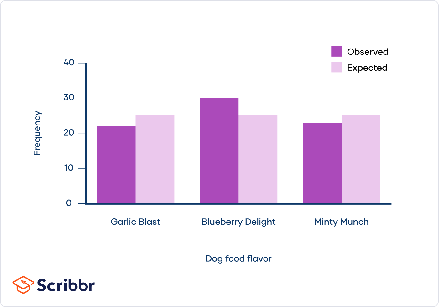
- Observed Frequencies: The actual data collected from the sample.
- Expected Frequencies: The frequencies that would be expected if there was no association between the variables.
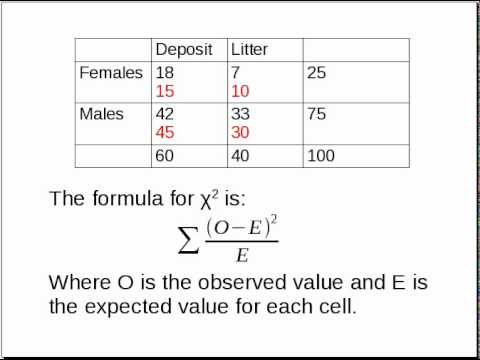
- Chi-Square Statistic: Calculated as
$$ \chi^2 = \sum \frac{(O_i - E_i)^2}{E_i} $$ , where \(O_i\) is the observed frequency and \(E_i\) is the expected frequency for each category.
The chi-square test is applicable in various scenarios, including:
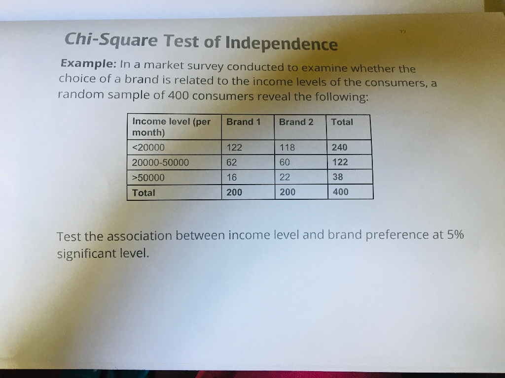
- Chi-Square Test for Independence: Used to determine if there is a significant association between two categorical variables in a contingency table.
- Chi-Square Goodness-of-Fit Test: Used to compare the observed distribution of a single categorical variable to a theoretical distribution.
Steps to conduct a chi-square test:
- Formulate the null hypothesis (\(H_0\)) stating that there is no association between the variables.
- Collect and organize the data into a contingency table.
- Calculate the expected frequencies for each cell in the table.
- Compute the chi-square statistic using the formula above.
- Determine the degrees of freedom (df) as \((r - 1) \times (c - 1)\), where \(r\) is the number of rows and \(c\) is the number of columns.
- Compare the calculated chi-square statistic to the critical value from the chi-square distribution table at the desired significance level (\(\alpha\)).
- Make a decision: If the chi-square statistic is greater than the critical value, reject the null hypothesis.
The chi-square test is a powerful tool for analyzing categorical data and can provide valuable insights into relationships and patterns within the data. Understanding and applying the correct sample size is essential for the accuracy and reliability of the test results.
Importance of Sample Size in Chi-Square Test
The sample size in a chi-square test is crucial for ensuring the accuracy and validity of the test results. An appropriate sample size helps in obtaining reliable estimates and achieving sufficient statistical power to detect meaningful differences or associations. Below are the key reasons why sample size is important in a chi-square test:
- Accuracy of Expected Frequencies: For the chi-square test to be valid, the expected frequencies in each cell of the contingency table should ideally be 5 or more. A small sample size can lead to expected frequencies that are too low, compromising the test's validity.
- Statistical Power: The power of a chi-square test, defined as \(1 - \beta\), is the probability of correctly rejecting the null hypothesis when it is false. Adequate sample size ensures higher statistical power, reducing the risk of Type II errors (failing to detect a true effect).
- Effect Size Detection: Larger sample sizes are required to detect smaller effect sizes. The sample size should be sufficient to identify the strength of the association between variables.
Factors Influencing Sample Size Determination:
- Significance Level (\(\alpha\)): The probability of rejecting the null hypothesis when it is true (Type I error). Commonly used significance levels are 0.05, 0.01, and 0.10. A smaller \(\alpha\) requires a larger sample size.
- Power (\(1 - \beta\)): The probability of correctly rejecting the null hypothesis. A higher desired power level, such as 0.80 or 0.90, necessitates a larger sample size.
- Effect Size (\(\phi\)): The magnitude of the association between variables. The effect size can be calculated using the formula:
$$ \phi = \sqrt{\frac{\chi^2}{n}} $$ , where \( \chi^2 \) is the chi-square statistic and \( n \) is the sample size. Smaller effect sizes require larger sample sizes to be detected. - Degrees of Freedom (df): Calculated as \((r - 1) \times (c - 1)\), where \(r\) is the number of rows and \(c\) is the number of columns in the contingency table. More degrees of freedom typically require a larger sample size.
Practical Steps to Determine Sample Size:
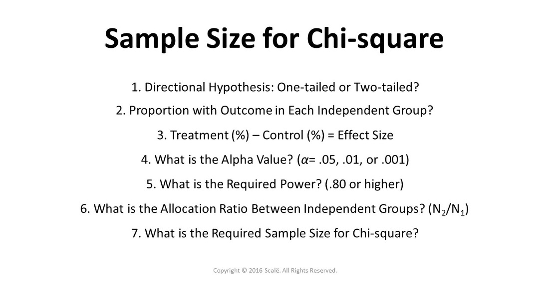
- Define the significance level (\(\alpha\)), desired power (\(1 - \beta\)), and estimated effect size (\(\phi\)).
- Calculate the degrees of freedom based on the structure of the contingency table.
- Use statistical software or sample size calculation formulas to determine the required sample size.
For example, one commonly used formula for sample size calculation is:
$$
n = \left( \frac{(Z_{\alpha/2} + Z_{\beta})^2 \cdot (r - 1) \cdot (c - 1)}{\phi^2} \right)
$$
In summary, an adequate sample size is essential for the reliability and validity of chi-square test results. It ensures that the expected frequencies are sufficient, increases the test's power, and enables the detection of meaningful effect sizes. Careful consideration of the factors influencing sample size determination and using appropriate calculation methods are key to successful chi-square test implementation.
Factors Influencing Sample Size Determination
Determining the appropriate sample size for a chi-square test is critical to ensure the validity and reliability of the test results. Several factors influence the calculation of sample size, and understanding these factors helps in designing robust studies. Below are the key factors:
- Effect Size:
Effect size refers to the magnitude of the difference or association being tested. Larger effect sizes generally require smaller sample sizes to detect, while smaller effect sizes require larger sample sizes. Effect size can be quantified using measures such as Cohen's w for chi-square tests.
- Significance Level (Alpha):
The significance level, denoted as α, is the probability of rejecting the null hypothesis when it is true (Type I error). Commonly used values for α are 0.05, 0.01, and 0.10. Lower α levels (e.g., 0.01) require larger sample sizes to maintain the same power.
- Power of the Test (1 - Beta):
The power of a test, represented as 1 - β, is the probability of correctly rejecting the null hypothesis when it is false (avoiding Type II error). Higher power (e.g., 0.80 or 0.90) necessitates larger sample sizes. Power analysis is crucial in sample size determination.
- Degrees of Freedom (df):
Degrees of freedom in a chi-square test are determined by the number of categories being analyzed. For a test of independence, df is calculated as (rows - 1) * (columns - 1). Higher degrees of freedom generally increase the required sample size.
- Expected Frequencies:
The expected frequencies in each cell of a contingency table should ideally be 5 or more for the chi-square test to be valid. If expected frequencies are low, increasing the sample size is necessary to meet this criterion.
- Population Variability:
Greater variability in the population requires a larger sample size to detect significant differences. Less variability means a smaller sample size may be sufficient.
- Design Effect:
In complex survey designs (e.g., stratified, clustered sampling), the design effect accounts for the increased variance. The design effect (Deff) is used to adjust the sample size:
n_{adj} = n \times Deff , wheren_{adj} is the adjusted sample size.
Considering these factors comprehensively ensures an adequate sample size for achieving reliable and valid results in chi-square tests.
Calculating Expected Frequencies
To perform a chi-square test, it's crucial to calculate the expected frequencies. The expected frequency is the frequency we would expect in each category if there were no association between the variables. Here's a step-by-step guide to calculating expected frequencies:
-
Create a Contingency Table: Start by arranging your data into a contingency table, which shows the frequency of occurrences for combinations of categorical variables.
Category 1 Category 2 Category 3 Total Group A 15 12 9 36 Group B 8 8 6 22 Total 23 20 15 58 -
Calculate Row and Column Totals: Sum the rows and columns to get the totals. These totals will be used in the expected frequency formula.
-
Use the Expected Frequency Formula: The formula to calculate the expected frequency for each cell in the table is:
\[ E_{ij} = \frac{(R_i \cdot C_j)}{N} \]
Where:
- \( E_{ij} \) = expected frequency for the cell in the ith row and jth column
- \( R_i \) = total for the ith row
- \( C_j \) = total for the jth column
- \( N \) = grand total of all observations
-
Calculate Each Expected Frequency: Apply the formula to each cell in the table. For example, for the cell in the first row and first column:
\[ E_{11} = \frac{(36 \cdot 23)}{58} = 14.31 \]
-
Fill in the Expected Frequencies: Repeat the calculation for each cell in the table:
Category 1 Category 2 Category 3 Total Group A 14.31 12.41 9.29 36 Group B 8.69 7.59 5.71 22 Total 23 20 15 58
By calculating these expected frequencies, you can proceed with the chi-square test to compare them with the observed frequencies and determine if there is a significant difference.

Effect Size and Its Impact on Sample Size
Effect size is a critical factor in determining the required sample size for a chi-square test. It measures the magnitude of the association between variables, helping to interpret the practical significance of the results. In chi-square tests, common effect size measures include Phi (φ) and Cramer's V.
- Phi (φ): Suitable for 2x2 contingency tables.
- Formula: \( \phi = \sqrt{\frac{\chi^2}{n}} \)
- Interpretation:
- Small effect: \( \phi = 0.1 \)
- Medium effect: \( \phi = 0.3 \)
- Large effect: \( \phi = 0.5 \)
- Cramer's V: Used for larger tables.
- Formula: \( V = \sqrt{\frac{\chi^2}{n \cdot \min(k-1, r-1)}} \)
- Interpretation depends on degrees of freedom (df):
- For df = 1: Small \( V = 0.1 \), Medium \( V = 0.3 \), Large \( V = 0.5 \)
- For df = 2: Small \( V = 0.07 \), Medium \( V = 0.21 \), Large \( V = 0.35 \)
- For df = 3: Small \( V = 0.06 \), Medium \( V = 0.17 \), Large \( V = 0.29 \)
The effect size influences the sample size needed to achieve a given level of statistical power. Larger effect sizes require smaller sample sizes to detect a significant effect, while smaller effect sizes require larger sample sizes. The following steps illustrate how to calculate the sample size based on effect size:
- Determine the desired effect size (φ or V): Use prior research or pilot studies to estimate an expected effect size.
- Select the significance level (α): Common choices are 0.05 or 0.01.
- Choose the power of the test (1 - β): Typically set at 0.80 or 0.90.
- Calculate the sample size: Use statistical software or sample size tables that incorporate the effect size, significance level, and power.
Understanding the relationship between effect size and sample size helps researchers design studies that are both efficient and statistically sound. By ensuring the sample size is adequate to detect meaningful differences, researchers can draw more reliable conclusions from their chi-square tests.
Significance Level (Alpha) and Its Role
The significance level, denoted as \(\alpha\), is a critical component in hypothesis testing. It represents the probability of rejecting the null hypothesis when it is actually true, known as a Type I error. Typically, common significance levels are 0.05 (5%) and 0.01 (1%). Here's a detailed breakdown of its role in the chi-square test:
1. Setting the Significance Level
Before conducting a chi-square test, the significance level must be set. This predetermined threshold helps in deciding whether to reject the null hypothesis. The choice of \(\alpha\) influences the probability of making a Type I error.
2. Comparing P-Value with Alpha
After calculating the chi-square statistic, we obtain a p-value. This p-value is compared with the chosen \(\alpha\). The decision rules are:
- If \( p \leq \alpha \), reject the null hypothesis.
- If \( p > \alpha \), do not reject the null hypothesis.
This comparison determines if the observed data significantly deviates from the expected data under the null hypothesis.
3. Impact on Test Outcomes
The significance level directly affects the test's conclusions:
- Lower \(\alpha\): More stringent criteria for rejecting the null hypothesis, reducing the chance of a Type I error but increasing the chance of a Type II error (failing to reject a false null hypothesis).
- Higher \(\alpha\): Less stringent criteria, increasing the chance of detecting an effect if one exists but also increasing the risk of a Type I error.
4. Example Calculation
Consider a chi-square test with a calculated p-value of 0.03 and \(\alpha\) set at 0.05:
- Since \( 0.03 \leq 0.05 \), we reject the null hypothesis.
- This indicates that there is a statistically significant difference between the observed and expected frequencies at the 5% significance level.
5. Practical Considerations
Choosing an appropriate \(\alpha\) depends on the context of the study. For critical applications, a lower \(\alpha\) (e.g., 0.01) might be preferred to minimize false positives. In exploratory research, a higher \(\alpha\) (e.g., 0.10) may be acceptable to ensure potential findings are not overlooked.
In summary, the significance level \(\alpha\) plays a crucial role in determining the reliability and validity of the conclusions drawn from a chi-square test. It balances the risk of Type I and Type II errors, influencing the overall decision-making process in statistical hypothesis testing.
Power of the Test (1 - Beta)
The power of a statistical test, denoted as \(1 - \beta\), is the probability that the test correctly rejects the null hypothesis when the alternative hypothesis is true. In other words, it measures the test's ability to detect an effect if there is one.
Several factors influence the power of a chi-square test:
- Sample Size (N): Larger sample sizes generally increase the power of the test. This is because larger samples provide more information and make it easier to detect a true effect.
- Effect Size (w): The magnitude of the difference or relationship that the test is trying to detect. Larger effect sizes increase the power of the test. Effect size for chi-square tests is often measured using Cohen's w, calculated as: \[ w = \sqrt{\frac{\sum (O_i - E_i)^2}{E_i \cdot N}} \] where \(O_i\) are the observed frequencies and \(E_i\) are the expected frequencies.
- Significance Level (\(\alpha\)): The probability of rejecting the null hypothesis when it is true (Type I error). A higher significance level increases power but also increases the risk of Type I error.
- Number of Categories (k): The number of categories or groups being compared. More categories can reduce power if the sample size is not increased proportionately.
To calculate the power of a chi-square test, you can use statistical software or specific formulas. One common approach is to use the non-central chi-square distribution to find the critical value for a given significance level and degrees of freedom.
Here is a step-by-step approach to determine the power of a chi-square test:
- Define the null and alternative hypotheses.
- Calculate the expected frequencies under the null hypothesis.
- Determine the observed frequencies from your sample data.
- Calculate the chi-square test statistic.
- Determine the degrees of freedom (df), typically calculated as \( (number \, of \, categories - 1) \).
- Using the non-central chi-square distribution, find the critical value for your significance level and degrees of freedom.
- Compare the calculated chi-square statistic to the critical value to decide whether to reject the null hypothesis.
- Calculate the non-centrality parameter (\(\lambda\)) using: \[ \lambda = N \times w^2 \] where \(N\) is the sample size and \(w\) is the effect size.
- Use the non-central chi-square distribution to find the power of the test given \(\lambda\), df, and \(\alpha\).
Software tools like R, Python, and specific statistical packages like G*Power or MATLAB provide functions to automate these calculations, allowing researchers to input parameters and receive power estimates.
Degrees of Freedom (df)
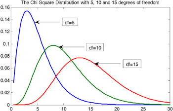
The degrees of freedom (df) in a chi-square test are crucial for determining the critical value needed to assess whether the observed data deviate significantly from the expected data. In the context of the chi-square test, the degrees of freedom depend on the specific test being conducted and the structure of the data.
Calculating Degrees of Freedom
For a chi-square test, the degrees of freedom are calculated differently based on the type of test:
- Chi-Square Test of Independence: Used to determine if there is a significant association between two categorical variables. The degrees of freedom are calculated as:
\[ df = (r - 1) \times (c - 1) \] where \(r\) is the number of rows and \(c\) is the number of columns in the contingency table. - Chi-Square Goodness of Fit Test: Used to determine if a sample data matches a population with a specific distribution. The degrees of freedom are calculated as:
\[ df = n - 1 \] where \(n\) is the number of categories or groups.
Example Calculation
Consider a study examining the relationship between recycling habits and different intervention methods (flyer, phone call, control). Suppose we have the following contingency table:
| Intervention | Recycles | Does Not Recycle |
|---|---|---|
| Flyer | 89 | 9 |
| Phone Call | 84 | 8 |
| Control | 86 | 24 |
The degrees of freedom for this chi-square test of independence are calculated as follows:
- Number of rows (\(r\)): 3 (Flyer, Phone Call, Control)
- Number of columns (\(c\)): 2 (Recycles, Does Not Recycle)
- Degrees of freedom:
\[ df = (3 - 1) \times (2 - 1) = 2 \]
Importance of Degrees of Freedom
Understanding the degrees of freedom is essential because it impacts the critical value against which the chi-square statistic is compared. A higher degree of freedom typically means a higher critical value, affecting the test's sensitivity to detect significant differences.
In summary, correctly calculating the degrees of freedom is a foundational step in conducting a chi-square test, ensuring accurate and reliable results.
Formula for Sample Size Calculation
Calculating the appropriate sample size for a chi-square test is crucial to ensure the validity of your statistical results. The sample size needed depends on several factors, including the effect size, the significance level (alpha), the power of the test, and the degrees of freedom. Below are the detailed steps to calculate the sample size for a chi-square test:
-
Determine the Effect Size (w)
The effect size (w) is a measure of the strength of the relationship between variables. It can be calculated using the formula:
\[
w = \sqrt{\frac{\chi^2}{N}}
\]where \(\chi^2\) is the chi-square statistic and \(N\) is the sample size.
-
Select the Significance Level (α)
The significance level (alpha) is the probability of rejecting the null hypothesis when it is true. Common values are 0.05, 0.01, and 0.10.
-
Choose the Desired Power (1 - β)
Power is the probability of correctly rejecting the null hypothesis when it is false. A commonly desired power level is 0.80.
-
Calculate the Degrees of Freedom (df)
The degrees of freedom for a chi-square test are calculated based on the number of categories in the variables being tested. For a chi-square test of independence, it is calculated as:
\[
df = (r - 1) \times (c - 1)
\]where \(r\) is the number of rows and \(c\) is the number of columns in the contingency table.
-
Use the Chi-Square Formula
To calculate the sample size, you can rearrange the formula for the chi-square statistic:
\[
N = \frac{\chi^2}{w^2}
\]Using a chi-square distribution table or software, find the critical value of \(\chi^2\) for the given degrees of freedom and significance level.
By following these steps, you can determine the necessary sample size to achieve reliable and valid results in your chi-square test.
Using Statistical Software for Sample Size Calculation
Statistical software packages can significantly simplify the process of calculating sample size for a Chi-Square test. These tools automate complex calculations and ensure accuracy. Here is a step-by-step guide on how to use statistical software for sample size calculation:
-
Select Your Software:
Choose a statistical software package that supports sample size calculation for Chi-Square tests. Popular options include SPSS, SAS, R, and online calculators.
-
Define Your Parameters:
- Effect Size (w): The magnitude of the effect you expect to detect. Small, medium, and large effect sizes are often represented by values of 0.1, 0.3, and 0.5 respectively.
- Significance Level (α): The probability of rejecting the null hypothesis when it is true. Common values are 0.05 or 0.01.
- Power (1 - β): The probability of correctly rejecting the null hypothesis. A common target value is 0.8 or 80%.
- Degrees of Freedom (df): Typically calculated as the product of the number of categories minus one for both variables in a contingency table (df = (r-1)(c-1)).
-
Input Data:
Enter the specified parameters into the software. For example, in SPSS, navigate to "Analyze" > "Nonparametric Tests" > "Chi-Square" and then enter the necessary values.
-
Run the Calculation:
Execute the function to compute the sample size. The software will use the provided parameters to calculate the minimum sample size required to achieve the desired power and significance level.
-
Review Results:
Examine the output provided by the software. It should include the calculated sample size along with other relevant statistics, such as the critical value of the Chi-Square distribution.
Using statistical software for sample size calculations not only saves time but also reduces the risk of manual calculation errors. These tools provide detailed outputs that can help in planning and interpreting your study effectively.
Practical Considerations in Sample Size Determination
Determining the appropriate sample size for a Chi-Square test involves several practical considerations. These factors ensure the validity and reliability of the test results. Here are key considerations:
- Expected Frequencies: Ensure that the expected frequency in each cell of the contingency table is at least 5. This helps to maintain the accuracy of the Chi-Square approximation. If more than 20% of cells have expected counts less than 5, consider combining categories or collecting more data.
- Sample Size: Larger sample sizes lead to more reliable results. However, very large samples can make even trivial differences statistically significant. Balance the need for accuracy with practical constraints such as time and resources.
- Random Sampling: The data should be collected using a random sampling method to avoid bias and to ensure that the sample is representative of the population.
- Independence of Observations: Ensure that the observations are independent. This means each individual or unit should only contribute once to the contingency table. Paired or matched samples violate this assumption.
- Mutually Exclusive Categories: Each subject or data point should fall into one and only one category. Overlapping categories can lead to inaccurate results.
- Practical Constraints: Consider logistical aspects such as the time available for data collection, budget constraints, and accessibility to the population being studied.
- Ethical Considerations: Ensure that the process of data collection adheres to ethical standards, protecting the privacy and consent of participants.
Balancing these factors helps in determining a feasible and effective sample size for conducting a Chi-Square test, ensuring both practical and statistical validity.
Balancing Cost and Feasibility
When determining the sample size for a chi-square test, it is crucial to balance cost and feasibility. Practical considerations include budget constraints, time limitations, and the availability of resources. Below are some key points to consider:
-
Budget Constraints:
The cost of data collection can be significant, especially for large sample sizes. It is essential to estimate the budget early in the planning phase and to explore ways to optimize data collection methods to stay within budget.
-
Time Limitations:
Time is often a limiting factor in research. Larger sample sizes require more time for data collection and analysis. Researchers should evaluate the time available for the study and ensure that the sample size is manageable within this timeframe.
-
Resource Availability:
Resources such as personnel, equipment, and software can limit the feasible sample size. Ensuring adequate resources are available is vital for collecting and processing the required data.
-
Data Quality:
While larger sample sizes can provide more reliable results, the quality of data is equally important. Researchers should balance the sample size with the ability to maintain high data quality.
-
Statistical Power:
Achieving the desired statistical power is essential. Researchers must consider the minimum sample size required to detect a meaningful effect, considering the expected effect size and significance level.
-
Ethical Considerations:
Collecting more data than necessary can be wasteful and raise ethical concerns. Researchers should aim to use the minimum sample size needed to achieve reliable results.
Balancing these factors involves making informed trade-offs. For instance, if the budget is limited, researchers might opt for a smaller sample size but use more sophisticated data analysis techniques to maximize the information gained from the available data.
In summary, practical considerations in sample size determination for a chi-square test require careful planning and balancing cost, time, resource availability, data quality, statistical power, and ethical considerations.
Adjusting for Data Loss or Non-Response
In any study, it's crucial to account for potential data loss or non-response to ensure that the final sample size is sufficient to detect a significant effect. Here are steps to adjust your sample size to mitigate these issues:
-
Estimate the Proportion of Expected Loss: Start by estimating the proportion of participants you expect to lose due to non-response or dropout. This can be denoted as \(W\), where \(W\) is the proportion of participants who will not complete the study or provide necessary data.
-
Calculate the Adjusted Sample Size: Adjust your initial sample size to account for the expected loss. If \(N\) is the initial sample size calculated without considering data loss, the adjusted sample size \(N^{**}\) can be calculated using the formula:
\[
N^{**} = \dfrac{N}{1 - W}
\]For instance, if you expect a 15% dropout rate (\(W = 0.15\)), and your initial sample size \(N\) is 200, the adjusted sample size would be:
\[
N^{**} = \dfrac{200}{1 - 0.15} = \dfrac{200}{0.85} \approx 236
\] -
Adjust for Noncompliance or Protocol Deviations: In addition to dropouts, participants may not adhere to the study protocol, which can dilute the treatment effect. To adjust for noncompliance, consider the proportions of participants who will not follow the protocol in each group. Let \(R_O\) represent the proportion of the treatment group who will discontinue the therapy, and \(R_I\) represent the proportion of the control group who will switch to a more effective therapy. Adjust the sample size using the formula:
\[
N^{*} = \dfrac{N}{(1 - R_O - R_I)^2}
\]For example, if you estimate that 20% of the control group will switch to active therapy (\(R_I = 0.20\)) and 10% of the treatment group will discontinue therapy (\(R_O = 0.10\)), and your initial sample size \(N\) is 200 per group, the adjusted sample size would be:
\[
N^{*} = \dfrac{200}{(1 - 0.20 - 0.10)^2} = \dfrac{200}{0.70^2} \approx 409 \text{ per group}
\] -
Iterative Process: Adjusting for data loss and non-response may require an iterative approach. After estimating the adjusted sample size, plot power curves and reconsider your assumptions. Iterate the process as necessary to ensure robustness of your sample size calculation.
By carefully adjusting your sample size for potential data loss and non-response, you can enhance the reliability and validity of your study results.
Case Studies and Examples
To better understand the application of the Chi-Square test, let's look at some illustrative case studies and examples. These will help clarify how to conduct the test and interpret the results in different scenarios.
Case Study 1: Gender and Buying Patterns
Imagine a scenario where we want to determine if there's a relationship between gender and the type of product purchased. We surveyed 40 individuals, split evenly between men and women, who chose between a pen and a pencil. The observed frequencies are tabulated below:
| Pen | Pencil | Total | |
|---|---|---|---|
| Men | 10 | 10 | 20 |
| Women | 10 | 10 | 20 |
| Total | 20 | 20 | 40 |
In this example, the Chi-Square test will likely show no significant difference, indicating no relationship between gender and the choice of product.
Case Study 2: Preference for Drinks by Gender
In a different survey, 52 individuals were given a choice between a soft drink and chocolate. The observed frequencies are as follows:
| Soft Drink | Chocolate | Total | |
|---|---|---|---|
| Men | 20 | 8 | 28 |
| Women | 6 | 18 | 24 |
| Total | 26 | 26 | 52 |
The Chi-Square test statistic in this case is significant, indicating a relationship between gender and the type of product chosen. Men significantly preferred soft drinks while women preferred chocolates.
Example: Education Level and Gender
A random sample of 395 people was surveyed to determine if there's a relationship between gender and education level. The data collected is summarized in the following contingency table:
| High School | Bachelors | Masters | Ph.D. | Total | |
|---|---|---|---|---|---|
| Female | 60 | 54 | 46 | 41 | 201 |
| Male | 40 | 44 | 53 | 57 | 194 |
| Total | 100 | 98 | 99 | 98 | 395 |
Using the Chi-Square test, we calculate the expected frequencies and compare them with the observed values. The test statistic is significant, indicating that education level is dependent on gender at a 5% significance level.
Calculation of Chi-Square Statistic
The formula for the Chi-Square test statistic is:
\[
\chi^2 = \sum \frac{(O_i - E_i)^2}{E_i}
\]
Where \(O_i\) is the observed frequency and \(E_i\) is the expected frequency, calculated as:
\[
E_i = \frac{(\text{row total} \times \text{column total})}{\text{grand total}}
\]
This formula is applied to each cell in the contingency table, and the results are summed to obtain the Chi-Square test statistic.
Common Mistakes in Sample Size Calculation
When conducting a chi-square test, ensuring the appropriate sample size is crucial for accurate results. Here are common mistakes to avoid in sample size calculation:
-
Ignoring Minimum Cell Counts:
A common mistake is not ensuring that each expected cell count in the contingency table is at least 5. Small expected frequencies can invalidate the test's assumptions and lead to inaccurate conclusions.
-
Inappropriate Sample Size:
Using a sample size that is too small can lead to insufficient power, increasing the risk of a Type II error (failing to detect a real effect). Conversely, a sample size that is too large can detect trivial differences, leading to a Type I error (detecting an effect that is not real).
-
Misunderstanding Effect Size:
Failing to consider the effect size can result in a sample size that does not accurately reflect the practical significance of the findings. Effect size helps determine how large a sample is needed to detect a meaningful difference.
-
Ignoring the Influence of Alpha and Beta:
Alpha (the significance level) and beta (the probability of a Type II error) should both be considered when calculating sample size. Neglecting these can lead to incorrect estimations and unreliable results.
-
Overlooking Degrees of Freedom:
Degrees of freedom, calculated as
{ (r - 1)(c - 1) } where r is the number of rows and c is the number of columns, affect the chi-square distribution and the critical value. Incorrect degrees of freedom can lead to errors in hypothesis testing. -
Failing to Adjust for Non-Response:
Not accounting for potential non-response or data loss can lead to an underpowered study. It is essential to anticipate and adjust the sample size to compensate for expected dropouts.
To avoid these pitfalls, consider using statistical software for sample size calculations, which can account for these factors more accurately.
Advanced Topics and Further Reading
Delving deeper into the chi-square test, several advanced topics and resources can enhance your understanding and application of this statistical method. Below are some key areas and readings to consider:
-
Effect Size Measures:
Understanding effect size measures, such as Cramer's V and Phi coefficient, is crucial for interpreting the strength of the association in chi-square tests. These measures help quantify the importance of the results beyond mere statistical significance.
-
Assumptions and Limitations:
Chi-square tests come with specific assumptions, including the independence of observations and the requirement for expected frequencies to be sufficiently large (typically at least 5). Violating these assumptions can lead to inaccurate results. Alternatives like Fisher's Exact Test can be used when these conditions are not met.
-
Post Hoc Tests:
After finding a significant chi-square test, post hoc tests (such as pairwise z-tests) can identify which specific groups differ. These tests are essential for detailed analysis in studies with multiple categories.
-
Using Software for Advanced Analysis:
Statistical software like SPSS, R, and SAS provide advanced options for conducting and interpreting chi-square tests, including complex tables and post hoc analyses. Mastery of these tools can significantly enhance your analytical capabilities.
-
Goodness-of-Fit Tests:
Chi-square goodness-of-fit tests are used to determine if a sample data matches a population with a specific distribution. This application is vital in fields such as genetics and market research.
For further reading, consider the following resources:
-
Cohen, J. (1988). Statistical Power Analysis for the Social Sciences (2nd Edition). Hillsdale, New Jersey: Lawrence Erlbaum Associates.
-
Siegel, S., & Castellan, N.J. (1989). Nonparametric Statistics for the Behavioral Sciences (2nd ed.). Singapore: McGraw-Hill.
-
Warner, R.M. (2013). Applied Statistics (2nd Edition). Thousand Oaks, CA: SAGE.
-
Scaler Topics - Application of Chi Square Test: This comprehensive guide provides insights into various applications of chi-square tests in fields like genetics, market research, sociology, and more.
-
SPSS Tutorials - Chi-Square Goodness-of-Fit Test: This tutorial offers detailed guidance on performing and interpreting chi-square goodness-of-fit tests using SPSS, complete with practical examples and syntax.

Chi Square và Kích Thước Mẫu - Video hướng dẫn về cách tính kích thước mẫu cho kiểm định Chi Square, phù hợp cho bài viết với từ khóa 'chi square test sample size'.
Chi Square và Kích Thước Mẫu - Video Hướng Dẫn
READ MORE:
Kiểm Định Chi Square - Hướng dẫn chi tiết về kiểm định Chi Square và các ứng dụng trong thống kê. Phù hợp cho bài viết với từ khóa 'chi square test sample size'.
Kiểm Định Chi Square - Hướng Dẫn Cơ Bản

:max_bytes(150000):strip_icc()/Chi-SquareStatistic_Final_4199464-7eebcd71a4bf4d9ca1a88d278845e674.jpg)