Topic null hypothesis of chi square test: The null hypothesis of the chi-square test is a fundamental concept in statistical analysis, helping to determine the independence of categorical variables. This comprehensive guide will explain its definition, formulation, and applications, ensuring you grasp its importance and learn how to effectively apply it in your data analysis endeavors.
Table of Content
- Chi-Square Test of Independence
- Introduction to Chi-Square Test
- Definition of Null Hypothesis
- Formulating the Null Hypothesis in Chi-Square Test
- Types of Chi-Square Tests
- Chi-Square Test for Independence
- Chi-Square Goodness of Fit Test
- Assumptions of Chi-Square Test
- Steps in Conducting Chi-Square Test
- Calculating Chi-Square Statistic
- Interpreting Chi-Square Test Results
- Examples and Applications
- Common Misconceptions
- Limitations of Chi-Square Test
- YOUTUBE: Video hướng dẫn chi tiết về kiểm định chi-square và giả thuyết không, giúp bạn hiểu rõ cách thực hiện và áp dụng kiểm định này trong phân tích dữ liệu.
Chi-Square Test of Independence
The Chi-Square Test of Independence is a statistical test used to determine whether there is a significant association between two categorical variables. It is a nonparametric test, meaning it does not assume a normal distribution of the data.
Hypotheses
In the Chi-Square Test of Independence, the hypotheses are defined as follows:
- Null Hypothesis (H0): The two variables are independent, meaning there is no association between them.
- Alternative Hypothesis (H1): The two variables are not independent, meaning there is an association between them.
Formula
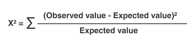
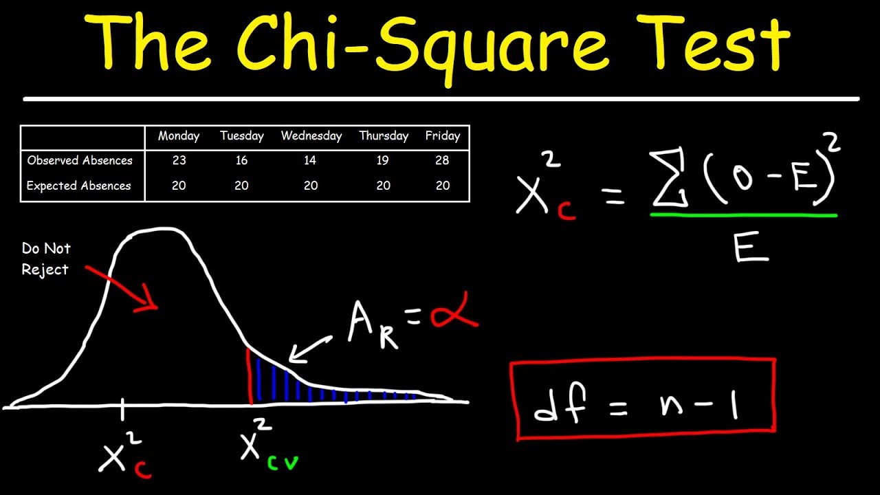
The test statistic for the Chi-Square test is calculated using the formula:
\[
\chi^2 = \sum \frac{(O_i - E_i)^2}{E_i}
\]
Where:
- \( O_i \) = Observed frequency
- \( E_i \) = Expected frequency
Steps to Perform Chi-Square Test
- Define the hypotheses.
- Calculate the expected frequencies for each category using the formula: \[ E = \frac{(\text{row total}) \times (\text{column total})}{\text{grand total}} \]
- Compute the Chi-Square statistic using the formula provided above.
- Determine the degrees of freedom: \[ \text{Degrees of freedom} = (r - 1) \times (c - 1) \] where \( r \) is the number of rows and \( c \) is the number of columns.
- Compare the computed Chi-Square statistic to the critical value from the Chi-Square distribution table at the desired significance level (e.g., 0.05).
- Make a decision: If the Chi-Square statistic is greater than the critical value, reject the null hypothesis.
Example
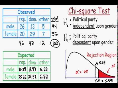
Suppose we want to determine if there is an association between gender and political party preference. We collect data from a sample of individuals and organize it into a contingency table:
| Gender | Republican | Democrat | Independent | Total |
|---|---|---|---|---|
| Male | 120 | 90 | 40 | 250 |
| Female | 110 | 95 | 45 | 250 |
| Total | 230 | 185 | 85 | 500 |
Based on the table, we calculate the expected frequencies and then use the Chi-Square formula to determine the test statistic.
Conclusion
If the p-value is less than the chosen significance level, we reject the null hypothesis and conclude that there is a significant association between the two variables. Otherwise, we fail to reject the null hypothesis.

READ MORE:
Introduction to Chi-Square Test
The chi-square test is a statistical method used to determine if there is a significant association between categorical variables. It is commonly applied in hypothesis testing to evaluate whether observed data deviate from expected data based on a specific hypothesis. The test is valuable in various fields, including research, business, and social sciences.
There are two main types of chi-square tests:
- Chi-Square Test for Independence
- Chi-Square Goodness of Fit Test
Both tests involve comparing the observed frequencies in the data to the frequencies expected under the null hypothesis.
The chi-square test for independence assesses whether two categorical variables are independent. In contrast, the goodness of fit test evaluates how well an observed frequency distribution matches an expected distribution.
The chi-square statistic is calculated using the formula:
\[
\chi^2 = \sum \frac{(O_i - E_i)^2}{E_i}
\]
where:
- \(O_i\) = observed frequency
- \(E_i\) = expected frequency
The steps to perform a chi-square test are as follows:
- Formulate the null and alternative hypotheses.
- Construct a contingency table (for independence) or a table of observed and expected frequencies (for goodness of fit).
- Calculate the expected frequencies.
- Compute the chi-square statistic using the formula above.
- Determine the degrees of freedom and find the critical value from the chi-square distribution table.
- Compare the chi-square statistic to the critical value to decide whether to reject the null hypothesis.
If the calculated chi-square statistic is greater than the critical value, the null hypothesis is rejected, indicating a significant association between the variables.
Definition of Null Hypothesis
The null hypothesis (\(H_0\)) is a fundamental concept in statistical hypothesis testing. It represents a statement of no effect or no difference, serving as a baseline or default position that researchers aim to test against. In the context of the chi-square test, the null hypothesis typically states that there is no significant association between the categorical variables being analyzed.
For example, in a chi-square test for independence, the null hypothesis can be formulated as:
\[
H_0: \text{The variables } X \text{ and } Y \text{ are independent.}
\]
In the chi-square goodness of fit test, the null hypothesis might be stated as:
\[
H_0: \text{The observed frequencies follow the expected distribution.}
\]
To test the null hypothesis, follow these steps:
- Define the null and alternative hypotheses.
- Collect and categorize the data into observed frequencies.
- Calculate the expected frequencies based on the null hypothesis.
- Compute the chi-square statistic using the formula: \[ \chi^2 = \sum \frac{(O_i - E_i)^2}{E_i} \]
- Determine the degrees of freedom, which is typically calculated as: \[ \text{Degrees of Freedom} = (r-1) \times (c-1) \] where \(r\) is the number of rows and \(c\) is the number of columns in the contingency table.
- Compare the chi-square statistic to the critical value from the chi-square distribution table.
- Make a decision:
- If the chi-square statistic is greater than the critical value, reject the null hypothesis.
- If the chi-square statistic is less than or equal to the critical value, do not reject the null hypothesis.
Rejecting the null hypothesis suggests that there is a significant association between the variables or that the observed frequencies significantly differ from the expected frequencies. Not rejecting the null hypothesis indicates that there is insufficient evidence to support a significant association or difference.
Formulating the Null Hypothesis in Chi-Square Test
Formulating the null hypothesis (\(H_0\)) in a chi-square test involves stating that there is no significant relationship or difference between the categorical variables being analyzed. The exact formulation depends on the type of chi-square test being conducted: the chi-square test for independence or the chi-square goodness of fit test.
Chi-Square Test for Independence
In a chi-square test for independence, the null hypothesis asserts that two categorical variables are independent of each other. For example, if you are examining whether there is a relationship between gender and voting preference, the null hypothesis would be:
\[
H_0: \text{Gender and voting preference are independent.}
\]
The alternative hypothesis (\(H_A\)) would be:
\[
H_A: \text{Gender and voting preference are not independent.}
\]
Chi-Square Goodness of Fit Test
In a chi-square goodness of fit test, the null hypothesis states that the observed frequency distribution matches an expected distribution. For instance, if you are testing whether a die is fair, the null hypothesis would be:
\[
H_0: \text{The die is fair (each face has an equal probability of 1/6).}
\]
The alternative hypothesis (\(H_A\)) would be:
\[
H_A: \text{The die is not fair (the faces do not have equal probabilities).}
\]
Steps to Formulate the Null Hypothesis
- Identify the categorical variables to be analyzed.
- Determine the type of chi-square test to be used: independence or goodness of fit.
- State the null hypothesis (\(H_0\)) clearly, indicating no significant association or difference.
- Formulate the alternative hypothesis (\(H_A\)), indicating a significant association or difference.
Examples
Here are some examples of formulating null hypotheses for different scenarios:
- Independence Test: Testing the relationship between education level and job satisfaction.
- \(H_0\): Education level and job satisfaction are independent.
- \(H_A\): Education level and job satisfaction are not independent.
- Goodness of Fit Test: Testing if the distribution of colors in a bag of M&Ms matches the company's stated proportions.
- \(H_0\): The observed color distribution matches the expected distribution.
- \(H_A\): The observed color distribution does not match the expected distribution.
Formulating the null hypothesis is a crucial step in the chi-square test as it sets the foundation for statistical testing and interpretation of results.
Types of Chi-Square Tests
The chi-square test is a versatile statistical tool used to examine the relationship between categorical variables. There are two main types of chi-square tests, each serving different purposes: the Chi-Square Test for Independence and the Chi-Square Goodness of Fit Test.
Chi-Square Test for Independence
The Chi-Square Test for Independence is used to determine whether there is a significant association between two categorical variables. This test assesses if the distribution of one variable is independent of the distribution of another variable. It is commonly applied in research fields such as social sciences, marketing, and health studies.
Steps to perform the Chi-Square Test for Independence:
- Formulate the hypotheses:
- Null hypothesis (\(H_0\)): The two variables are independent.
- Alternative hypothesis (\(H_A\)): The two variables are not independent.
- Construct a contingency table to display the frequencies of the variables.
- Calculate the expected frequencies for each cell in the table using the formula: \[ E_{ij} = \frac{( \text{Row total}_i \times \text{Column total}_j )}{\text{Grand total}} \]
- Compute the chi-square statistic: \[ \chi^2 = \sum \frac{(O_{ij} - E_{ij})^2}{E_{ij}} \] where \(O_{ij}\) is the observed frequency and \(E_{ij}\) is the expected frequency.
- Determine the degrees of freedom: \[ \text{Degrees of Freedom} = (r-1) \times (c-1) \] where \(r\) is the number of rows and \(c\) is the number of columns.
- Compare the chi-square statistic to the critical value from the chi-square distribution table to decide whether to reject the null hypothesis.
Chi-Square Goodness of Fit Test
The Chi-Square Goodness of Fit Test evaluates how well the observed frequency distribution of a single categorical variable matches an expected distribution. This test is often used to test hypotheses about the distribution of a categorical variable in a population.
Steps to perform the Chi-Square Goodness of Fit Test:
- Formulate the hypotheses:
- Null hypothesis (\(H_0\)): The observed frequencies match the expected frequencies.
- Alternative hypothesis (\(H_A\)): The observed frequencies do not match the expected frequencies.
- Collect and categorize the observed data.
- Calculate the expected frequencies based on the null hypothesis.
- Compute the chi-square statistic: \[ \chi^2 = \sum \frac{(O_i - E_i)^2}{E_i} \] where \(O_i\) is the observed frequency and \(E_i\) is the expected frequency.
- Determine the degrees of freedom: \[ \text{Degrees of Freedom} = k - 1 \] where \(k\) is the number of categories.
- Compare the chi-square statistic to the critical value from the chi-square distribution table to decide whether to reject the null hypothesis.
Understanding the types of chi-square tests and their applications is essential for accurately analyzing categorical data and drawing meaningful conclusions from statistical analyses.
:max_bytes(150000):strip_icc()/Chi-SquareStatistic_Final_4199464-7eebcd71a4bf4d9ca1a88d278845e674.jpg)
Chi-Square Test for Independence
The Chi-Square Test for Independence is a statistical test used to determine if there is a significant association between two categorical variables. It helps to understand whether the distribution of one variable is independent of the distribution of another variable. This test is widely used in various fields such as social sciences, biology, and marketing.
Steps to Perform Chi-Square Test for Independence
- Formulate the Hypotheses:
- Null Hypothesis (\(H_0\)): The two variables are independent.
- Alternative Hypothesis (\(H_A\)): The two variables are not independent.
- Collect Data and Construct a Contingency Table:
Organize the data into a contingency table, showing the frequency distribution of the variables.
Category 1 Category 2 Category 3 Row Totals Group A Observed Frequency (O11) Observed Frequency (O12) Observed Frequency (O13) Row Total Group B Observed Frequency (O21) Observed Frequency (O22) Observed Frequency (O23) Row Total Group C Observed Frequency (O31) Observed Frequency (O32) Observed Frequency (O33) Row Total Column Totals Column Total Column Total Column Total Grand Total - Calculate Expected Frequencies:
The expected frequency for each cell is calculated using the formula:
\[
E_{ij} = \frac{(\text{Row total}_i \times \text{Column total}_j)}{\text{Grand total}}
\] - Compute the Chi-Square Statistic:
Calculate the chi-square statistic using the formula:
\[
\chi^2 = \sum \frac{(O_{ij} - E_{ij})^2}{E_{ij}}
\]where \(O_{ij}\) is the observed frequency and \(E_{ij}\) is the expected frequency.
- Determine the Degrees of Freedom:
The degrees of freedom for the test is calculated as:
\[
\text{Degrees of Freedom} = (r-1) \times (c-1)
\]where \(r\) is the number of rows and \(c\) is the number of columns in the contingency table.
- Compare the Chi-Square Statistic to the Critical Value:
Using the degrees of freedom, find the critical value from the chi-square distribution table. Compare the calculated chi-square statistic to the critical value.
- If the chi-square statistic is greater than the critical value, reject the null hypothesis (\(H_0\)).
- If the chi-square statistic is less than or equal to the critical value, do not reject the null hypothesis (\(H_0\)).
By following these steps, you can determine whether there is a significant association between the two categorical variables. If the null hypothesis is rejected, it indicates that the variables are not independent and there is a significant relationship between them.
Chi-Square Goodness of Fit Test
The Chi-Square Goodness of Fit Test is a statistical test used to determine whether the observed frequency distribution of a categorical variable matches an expected distribution. This test is useful for testing hypotheses about the distribution of a single categorical variable in a population.
Steps to Perform Chi-Square Goodness of Fit Test
- Formulate the Hypotheses:
- Null Hypothesis (\(H_0\)): The observed frequencies match the expected frequencies.
- Alternative Hypothesis (\(H_A\)): The observed frequencies do not match the expected frequencies.
- Collect and Categorize the Data:
Gather the observed data and categorize it into appropriate bins or categories.
- Calculate Expected Frequencies:
The expected frequency for each category is calculated based on the null hypothesis. For example, if you are testing whether a die is fair, the expected frequency for each face (1 through 6) would be:
\[
E_i = \frac{\text{Total number of rolls}}{6}
\] - Compute the Chi-Square Statistic:
Calculate the chi-square statistic using the formula:
\[
\chi^2 = \sum \frac{(O_i - E_i)^2}{E_i}
\]where \(O_i\) is the observed frequency and \(E_i\) is the expected frequency.
- Determine the Degrees of Freedom:
The degrees of freedom for the test is calculated as:
\[
\text{Degrees of Freedom} = k - 1
\]where \(k\) is the number of categories.
- Compare the Chi-Square Statistic to the Critical Value:
Using the degrees of freedom, find the critical value from the chi-square distribution table. Compare the calculated chi-square statistic to the critical value.
- If the chi-square statistic is greater than the critical value, reject the null hypothesis (\(H_0\)).
- If the chi-square statistic is less than or equal to the critical value, do not reject the null hypothesis (\(H_0\)).
Example
Consider an example where you want to test whether a six-sided die is fair. You roll the die 60 times and observe the following frequencies:
| Face | Observed Frequency (Oi) | Expected Frequency (Ei) |
| 1 | 10 | 10 |
| 2 | 8 | 10 |
| 3 | 12 | 10 |
| 4 | 11 | 10 |
| 5 | 9 | 10 |
| 6 | 10 | 10 |
The chi-square statistic is calculated as follows:
\[
\chi^2 = \sum \frac{(O_i - E_i)^2}{E_i} = \frac{(10-10)^2}{10} + \frac{(8-10)^2}{10} + \frac{(12-10)^2}{10} + \frac{(11-10)^2}{10} + \frac{(9-10)^2}{10} + \frac{(10-10)^2}{10} = 0 + 0.4 + 0.4 + 0.1 + 0.1 + 0 = 1
\]
With 5 degrees of freedom (6 categories - 1), compare the chi-square statistic to the critical value from the chi-square distribution table. If the chi-square statistic is less than or equal to the critical value, you do not reject the null hypothesis, indicating that the die is fair. Otherwise, you reject the null hypothesis, suggesting that the die is not fair.
The Chi-Square Goodness of Fit Test is a powerful tool for assessing how well an observed distribution matches an expected distribution, providing valuable insights into the nature of categorical data.
Assumptions of Chi-Square Test
The Chi-Square Test is a widely used statistical method, but it relies on several key assumptions to ensure the validity of its results. Understanding and meeting these assumptions is crucial for accurate interpretation of the test outcomes.
Key Assumptions of Chi-Square Test
- Independence of Observations:
Each observation should be independent of the others. This means that the occurrence of one event should not affect the occurrence of another. In a contingency table, this implies that the data should be collected in such a way that there is no overlap between categories.
- Large Sample Size:
The chi-square test requires a sufficiently large sample size to ensure that the expected frequency in each cell of the contingency table is adequate. Typically, the expected frequency should be at least 5 for each cell. If the sample size is too small, the test may not be valid.
- Categorical Data:
The chi-square test is designed for categorical data, not continuous data. The data should be organized into categories, such as "yes" or "no" responses, or different levels of a factor.
- Expected Frequency:
Each expected frequency in the contingency table should be at least 5. If this condition is not met, the validity of the test can be compromised. For smaller sample sizes or when expected frequencies are less than 5, it is recommended to use Fisher's Exact Test instead.
- Mutually Exclusive Categories:
The categories for each variable should be mutually exclusive. This means that each observation should fall into one and only one category, ensuring clear distinctions between the categories.
Example of Checking Assumptions
Consider a study examining the relationship between smoking status (smoker, non-smoker) and the presence of a certain health condition (yes, no). To use the chi-square test, ensure the following:
- Independence: Each participant's smoking status and health condition are recorded independently of others.
- Large Sample Size: The study includes a sufficiently large number of participants to ensure that the expected frequency in each cell is at least 5.
- Categorical Data: Both smoking status and health condition are categorical variables.
- Expected Frequency: Calculate the expected frequencies to ensure they meet the minimum requirement of 5 per cell.
- Mutually Exclusive Categories: Each participant is classified as either a smoker or non-smoker, and either has the health condition or does not, with no overlap.
Conclusion
Meeting the assumptions of the chi-square test is essential for accurate and reliable results. By ensuring independence of observations, a large sample size, categorical data, adequate expected frequencies, and mutually exclusive categories, researchers can confidently use the chi-square test to analyze associations between categorical variables.
Steps in Conducting Chi-Square Test
Conducting a Chi-Square Test involves several steps to ensure the accuracy and reliability of the results. Below are the detailed steps:
-
Formulate the Hypotheses:
Define the null hypothesis (\( H_0 \)) and the alternative hypothesis (\( H_1 \)). The null hypothesis typically states that there is no significant difference or association between the observed and expected frequencies.
-
Collect and Organize Data:
Gather the observed frequencies from the data and organize them into a contingency table or frequency table as required.
-
Calculate the Expected Frequencies:
Using the marginal totals of the contingency table, calculate the expected frequencies for each cell. The formula for expected frequency (\( E \)) in a cell is:
E = \frac{(\text{Row Total} \times \text{Column Total})}{\text{Grand Total}} -
Compute the Chi-Square Statistic:
Use the formula to calculate the Chi-Square statistic (\( \chi^2 \)):
\( \chi^2 = \sum \frac{(O - E)^2}{E} \)where \( O \) is the observed frequency and \( E \) is the expected frequency.
-
Determine the Degrees of Freedom:
Calculate the degrees of freedom (df) for the test. For a contingency table, the degrees of freedom is:
\text{df} = (\text{number of rows} - 1) \times (\text{number of columns} - 1) -
Find the Critical Value:
Using a Chi-Square distribution table, find the critical value corresponding to the calculated degrees of freedom and the chosen significance level (\( \alpha \)), typically 0.05.
-
Compare the Chi-Square Statistic to the Critical Value:
If the Chi-Square statistic is greater than the critical value, reject the null hypothesis. Otherwise, do not reject the null hypothesis.
-
Draw Conclusions:
Based on the comparison, conclude whether there is sufficient evidence to reject the null hypothesis and accept the alternative hypothesis, indicating a significant difference or association.
Calculating Chi-Square Statistic
The Chi-Square statistic is calculated to determine if there is a significant difference between the expected and observed frequencies in one or more categories. Follow these detailed steps to calculate the Chi-Square statistic:
-
Set up the hypotheses:
- Null hypothesis (\(H_0\)): There is no significant difference between the expected and observed frequencies.
- Alternative hypothesis (\(H_1\)): There is a significant difference between the expected and observed frequencies.
-
Construct the contingency table:
Organize the data into a table that displays the observed frequencies for each category.
Category Observed Frequency (O) Expected Frequency (E) Category 1 O1 E1 Category 2 O2 E2 ... ... ... -
Calculate the expected frequencies:
For each category, the expected frequency (\(E\)) can be calculated using the formula:
\[
E = \frac{(\text{Row total} \times \text{Column total})}{\text{Grand total}}
\] -
Compute the Chi-Square statistic:
Use the formula to calculate the Chi-Square statistic:
\[
\chi^2 = \sum \frac{(O - E)^2}{E}
\]Where \(O\) represents the observed frequency and \(E\) represents the expected frequency.
-
Sum the calculated values:
Add up the values of \(\frac{(O - E)^2}{E}\) for each category to get the Chi-Square statistic.
-
Determine the degrees of freedom (df):
The degrees of freedom for the Chi-Square test are calculated as:
\[
\text{df} = (\text{Number of rows} - 1) \times (\text{Number of columns} - 1)
\] -
Compare the Chi-Square statistic to the critical value:
Using a Chi-Square distribution table, find the critical value for the calculated degrees of freedom and the chosen significance level (e.g., 0.05). If the Chi-Square statistic is greater than the critical value, reject the null hypothesis.
-
Draw a conclusion:
Based on the comparison, decide whether to reject or fail to reject the null hypothesis. If rejected, it suggests that there is a significant difference between the observed and expected frequencies.
This step-by-step approach ensures a thorough and accurate calculation of the Chi-Square statistic, allowing for proper statistical analysis and interpretation of categorical data.
Interpreting Chi-Square Test Results
Interpreting the results of a Chi-Square test involves several steps to determine whether there is a significant association between the categorical variables being studied. Below are the detailed steps:
-
Compare the Chi-Square Statistic to the Critical Value:
Once you have calculated the Chi-Square statistic (\(\chi^2\)), compare it to the critical value from the Chi-Square distribution table. The critical value depends on the degrees of freedom (df) and the chosen significance level (α), typically 0.05.
If \(\chi^2\) is greater than the critical value, you reject the null hypothesis (\(H_0\)). If \(\chi^2\) is less than or equal to the critical value, you do not reject the null hypothesis.
-
Determine the p-Value:
The p-value indicates the probability of obtaining a Chi-Square statistic at least as extreme as the one calculated, assuming the null hypothesis is true.
- If the p-value is less than the significance level (α), reject the null hypothesis.
- If the p-value is greater than or equal to the significance level, do not reject the null hypothesis.
-
Interpret the Results:
Based on the comparison, make a conclusion about the relationship between the variables:
- Reject the Null Hypothesis: There is evidence to suggest that there is a significant association between the variables.
- Fail to Reject the Null Hypothesis: There is no sufficient evidence to suggest a significant association between the variables.
-
Consider the Effect Size:
Beyond the p-value, consider the practical significance of the results by evaluating the effect size, which can provide insights into the strength of the association between the variables.
In summary, interpreting Chi-Square test results involves comparing the calculated statistic to critical values, analyzing the p-value, and making informed conclusions about the association between the variables. Always ensure the assumptions of the Chi-Square test are met for valid results.
Examples and Applications
The Chi-Square Test is a versatile statistical tool used across various fields to analyze categorical data. Below are some detailed examples and applications of the Chi-Square Test:
1. Chi-Square Test for Independence
This test determines whether there is a significant association between two categorical variables. For example, let's consider a study to investigate if there is a relationship between gender and political party preference among voters.
| Gender | Republican | Democrat | Independent | Total |
|---|---|---|---|---|
| Male | 120 | 90 | 40 | 250 |
| Female | 110 | 95 | 45 | 250 |
| Total | 230 | 185 | 85 | 500 |
Using the Chi-Square Test, we calculate the expected frequencies and then the Chi-Square statistic. The result helps us determine if the observed differences are statistically significant.
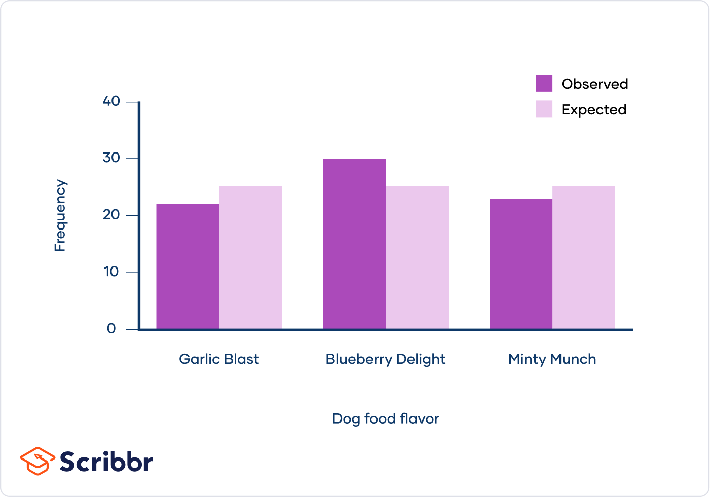
2. Chi-Square Goodness-of-Fit Test
This test is used to see if an observed frequency distribution differs from a theoretical distribution. For example, you might want to test if a bag of colored balls has an equal distribution of five different colors as expected.
Suppose we expect each color to appear 20% of the time in a bag of 100 balls:
- Red: 20
- Blue: 20
- Green: 20
- Yellow: 20
- Purple: 20
We can then compare the observed frequencies with these expected values to see if the distribution fits our expectation.
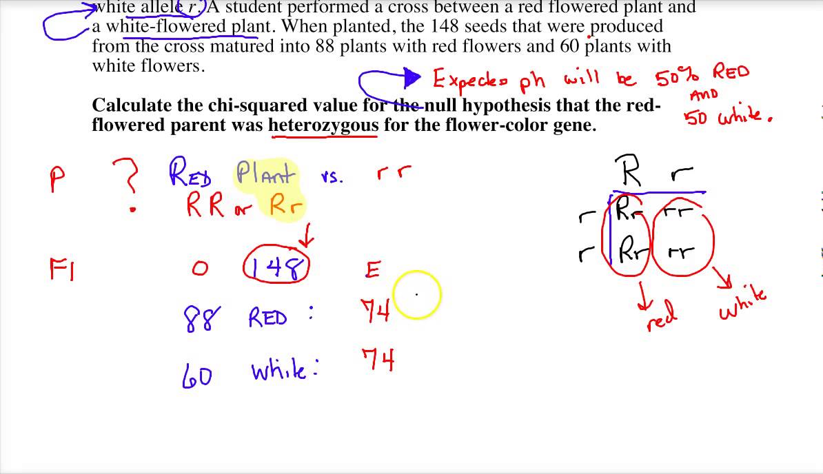
3. Application in Genetics
The Chi-Square Test is frequently used in genetics to determine if the distribution of traits follows expected Mendelian ratios. For instance, in a study of pea plants, the observed ratio of different traits (e.g., color and shape) can be compared against the expected 3:1 ratio predicted by Mendel's laws.
4. Marketing and Consumer Research
Marketers use the Chi-Square Test to analyze consumer preferences and behaviors. For example, a company might want to know if there is a significant preference for a new product among different age groups.
By collecting data from surveys and creating a contingency table, the company can apply the Chi-Square Test to see if age groups show different preferences.
5. Quality Control in Manufacturing
In quality control, the Chi-Square Test helps in determining whether the number of defective items in a batch is significantly different from what is expected. This application is crucial for maintaining product standards and consistency.
Conclusion
The Chi-Square Test is a powerful tool for analyzing categorical data and uncovering significant patterns and relationships in various fields, including social sciences, genetics, marketing, and quality control.
Common Misconceptions
While the Chi-Square test is a powerful statistical tool, several misconceptions about its application and interpretation are prevalent. Understanding these misconceptions is crucial for accurate data analysis and interpretation.
-
Misconception 1: Chi-Square Tests Require Normal Distribution
Unlike many statistical tests, Chi-Square tests do not require the data to be normally distributed. They are non-parametric tests designed for categorical data, which can take on a limited number of values and are not expected to follow a normal distribution.
-
Misconception 2: Small Expected Frequencies are Acceptable
For the Chi-Square test to be valid, it is recommended that the expected frequency in each cell of a contingency table should be at least 5. If this assumption is violated, the test results might not be reliable, and other statistical methods, like Fisher's Exact Test, might be more appropriate.
-
Misconception 3: Large Sample Sizes Always Lead to Significant Results
While larger sample sizes can increase the power of the test, they do not inherently make results significant. Large samples can indeed detect small differences, but it is crucial to consider the practical significance and not just the statistical significance.
-
Misconception 4: Chi-Square Tests Only Apply to Two Variables
Although commonly used for testing the independence of two categorical variables, the Chi-Square test can be extended to more than two variables through techniques like the Chi-Square test of homogeneity or multi-way tables.
-
Misconception 5: Rejecting the Null Hypothesis Proves a Specific Alternative
Rejecting the null hypothesis in a Chi-Square test suggests there is a significant difference between the observed and expected frequencies. However, it does not confirm the exact nature or cause of this difference. Further analysis is required to understand the specific relationship between variables.
-
Misconception 6: Chi-Square Test Results are Immune to Data Collection Methods
The accuracy of Chi-Square test results heavily depends on proper data collection methods. Non-random sampling or biased data collection can lead to invalid conclusions, emphasizing the importance of good experimental design.
Limitations of Chi-Square Test
The Chi-Square test is a widely used statistical tool, but it has several limitations that researchers need to consider when interpreting results:
- Independence Assumption: The test assumes that observations are independent. Violations of this assumption, such as correlations between observations, can affect the validity of the test.
- Sample Size: The reliability of the Chi-Square test is compromised with small sample sizes or low expected cell frequencies. It is generally recommended to have at least 5 expected frequencies per cell.
- Sensitivity to Sample Composition: The test can be biased by imbalanced frequencies or empty cells, which can lead to inaccurate conclusions.
- Applicability to Categorical Data: The Chi-Square test is designed for categorical variables and is not suitable for continuous or ordinal data.
- Lack of Directionality or Magnitude: While the test can indicate an association between variables, it does not provide information on the strength, direction, or magnitude of the association.
- Type of Association: The test can identify associations but cannot determine the type of association or establish cause-and-effect relationships.
- Large Sample Bias: In large samples, even small deviations can result in statistically significant results that may not have practical significance.
- Multiple Comparisons: Conducting multiple Chi-Square tests on the same data set increases the likelihood of finding significant results by chance. Adjustments, such as the Bonferroni correction, may be necessary to address this issue.
- Interpretation Considerations: It is crucial to interpret Chi-Square test results in the context of the research question and not to equate statistical significance with practical importance.
Understanding these limitations is essential for accurate interpretation and application of the Chi-Square test results in research and decision-making processes.
Video hướng dẫn chi tiết về kiểm định chi-square và giả thuyết không, giúp bạn hiểu rõ cách thực hiện và áp dụng kiểm định này trong phân tích dữ liệu.
Kiểm Định Chi-Square
READ MORE:
Video hướng dẫn chi tiết về thống kê chi-square và kiểm định giả thuyết, giúp bạn hiểu rõ cách thực hiện và áp dụng kiểm định này trong thống kê AP.
Thống kê Chi-square cho kiểm định giả thuyết | Thống kê AP | Khan Academy