Topic null hypothesis for a chi square test: Discover the essential aspects of the null hypothesis for a chi-square test in this comprehensive guide. Learn how to formulate, test, and interpret the null hypothesis to enhance your statistical analysis skills. Dive into the world of chi-square tests and understand their importance in hypothesis testing.
Table of Content
- Chi-Square Test of Independence
- Introduction to Chi-Square Test
- Understanding the Null Hypothesis
- Importance of the Null Hypothesis in Chi-Square Test
- Formulating the Null Hypothesis
- Chi-Square Test Types
- Goodness of Fit Test
- Test of Independence
- Homogeneity Test
- Assumptions of Chi-Square Test
- Calculating Chi-Square Statistic
- Interpreting Chi-Square Results
- Rejecting or Failing to Reject the Null Hypothesis
- Common Misconceptions
- Applications of Chi-Square Test
- YOUTUBE: Video giới thiệu về thống kê Chi-square trong kiểm định giả thuyết, giải thích cách sử dụng trong thống kê AP và ứng dụng của nó.
Chi-Square Test of Independence
The Chi-Square Test of Independence is a statistical test used to determine if there is a significant association between two categorical variables.
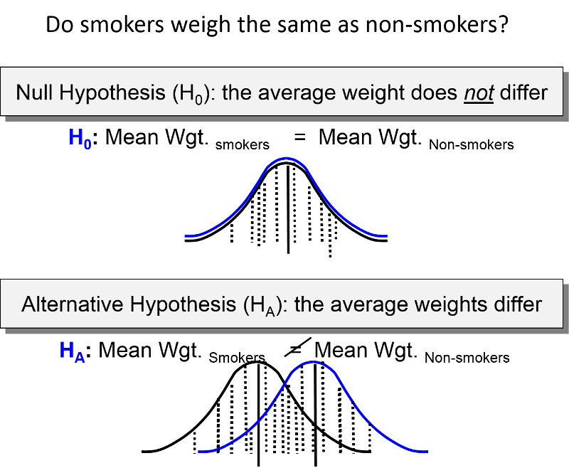
Hypotheses
The hypotheses for the Chi-Square Test of Independence are:
- Null Hypothesis (H0): The two categorical variables are independent.
- Alternative Hypothesis (H1): The two categorical variables are not independent.
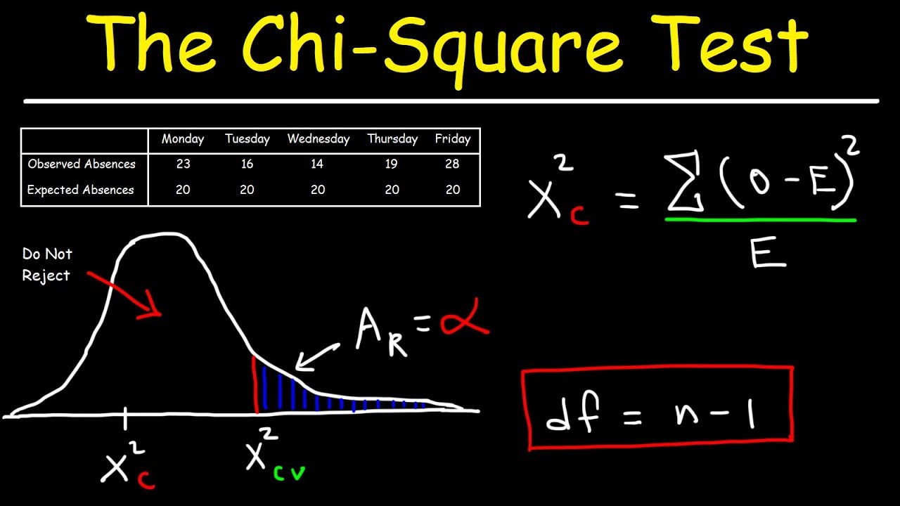
Test Statistic
The test statistic for the Chi-Square Test is calculated using the formula:
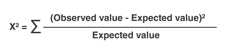
\[\chi^2 = \sum \frac{(O - E)^2}{E}\]
where \(O\) is the observed frequency and \(E\) is the expected frequency.
Steps to Perform the Test
- Define the hypotheses.
- Calculate the expected frequencies for each cell in the contingency table using the formula:
\[E = \frac{(\text{row total}) \times (\text{column total})}{\text{grand total}}\]
- Calculate the Chi-Square statistic using the formula provided.
- Determine the p-value associated with the calculated Chi-Square statistic and the degrees of freedom (df). Degrees of freedom are calculated as:
\[\text{df} = (r - 1) \times (c - 1)\]
where \(r\) is the number of rows and \(c\) is the number of columns.
- Compare the p-value to the significance level (usually 0.05) to decide whether to reject the null hypothesis.
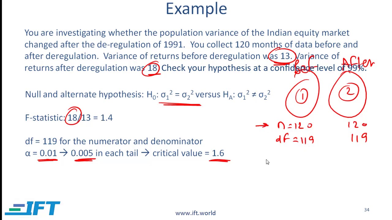
Example
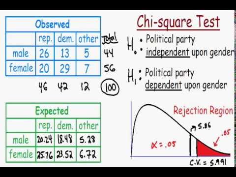
Consider an example where we test whether gender is associated with political party preference. The contingency table is:
| Republican | Democrat | Independent | Total | |
|---|---|---|---|---|
| Male | 120 | 90 | 40 | 250 |
| Female | 110 | 95 | 45 | 250 |
| Total | 230 | 185 | 85 | 500 |
Calculating the expected frequencies and then the Chi-Square statistic, we find:
\[\chi^2 = \sum \frac{(O - E)^2}{E} = 0.8642\]
With a p-value of 0.649198 and 2 degrees of freedom, we fail to reject the null hypothesis, indicating no significant association between gender and political party preference.
Conclusion
The Chi-Square Test of Independence helps determine if there is a significant relationship between two categorical variables by comparing observed and expected frequencies under the null hypothesis.
READ MORE:
Introduction to Chi-Square Test
The Chi-Square test is a statistical method used to determine if there is a significant association between categorical variables. It is widely used in hypothesis testing to assess whether observed data fits a particular theoretical distribution.
The Chi-Square test is divided into three main types:
- Goodness of Fit Test: This test determines if a sample data matches a population with a specific distribution.
- Test of Independence: This test evaluates if two categorical variables are independent of each other.
- Test of Homogeneity: This test compares the distribution of a categorical variable across different populations.
The formula for the Chi-Square statistic is:
\[
\chi^2 = \sum \frac{(O_i - E_i)^2}{E_i}
\]
where \( O_i \) is the observed frequency and \( E_i \) is the expected frequency.
Steps to conduct a Chi-Square test:
- Formulate the Null Hypothesis (H0): Assume there is no significant difference or association between the variables.
- Calculate the Expected Frequencies: Based on the null hypothesis, calculate the expected frequencies for each category.
- Compute the Chi-Square Statistic: Use the formula to calculate the Chi-Square value.
- Determine the Degrees of Freedom: Calculate the degrees of freedom, which depend on the number of categories.
- Find the P-Value: Compare the Chi-Square statistic to the Chi-Square distribution to obtain the p-value.
- Make a Decision: Reject or fail to reject the null hypothesis based on the p-value and the chosen significance level (usually 0.05).
The Chi-Square test is a powerful tool for analyzing categorical data and can provide valuable insights into the relationships between variables.
Understanding the Null Hypothesis
The null hypothesis (\(H_0\)) is a fundamental concept in statistical hypothesis testing. It represents a statement of no effect, no difference, or no association between variables. In the context of a chi-square test, the null hypothesis typically states that there is no significant association between the categorical variables being studied.
Formulating the null hypothesis involves the following steps:
- Identify the Variables: Determine the categorical variables that are being analyzed.
- State the Null Hypothesis: Construct a clear and concise statement that specifies there is no relationship or difference between the variables. For example, in a test of independence, the null hypothesis might be stated as, "There is no association between variable A and variable B."
In mathematical terms, the null hypothesis can be expressed as:
\[
H_0: O_i = E_i
\]
where \(O_i\) represents the observed frequencies and \(E_i\) represents the expected frequencies under the null hypothesis.
The null hypothesis is tested against an alternative hypothesis (\(H_a\)), which states that there is a significant association between the variables. The alternative hypothesis is usually formulated as:
\[
H_a: O_i \neq E_i
\]
In a chi-square test, the goal is to determine whether the observed data significantly deviates from the expected data under the null hypothesis. The steps to evaluate the null hypothesis are as follows:
- Calculate Expected Frequencies: Based on the null hypothesis, calculate the expected frequencies for each category.
- Compute the Chi-Square Statistic: Use the chi-square formula:
\[
\chi^2 = \sum \frac{(O_i - E_i)^2}{E_i}
\] - Determine the Degrees of Freedom: The degrees of freedom for a chi-square test are calculated as:
\[
\text{Degrees of Freedom} = (r - 1) \times (c - 1)
\]
where \(r\) is the number of rows and \(c\) is the number of columns in the contingency table. - Compare to Critical Value: Compare the calculated chi-square statistic to the critical value from the chi-square distribution table at a chosen significance level (typically 0.05).
- Make a Decision: If the chi-square statistic exceeds the critical value, reject the null hypothesis; otherwise, fail to reject the null hypothesis.
Understanding and correctly formulating the null hypothesis is crucial for conducting accurate and meaningful chi-square tests. It serves as the foundation for statistical inference and decision-making in hypothesis testing.
Importance of the Null Hypothesis in Chi-Square Test
The null hypothesis (\(H_0\)) is a cornerstone of the chi-square test, providing a basis for statistical inference and decision-making. Its importance can be understood through several key aspects:
- Foundation for Hypothesis Testing: The null hypothesis sets the stage for hypothesis testing by establishing a baseline assumption. It asserts that any observed differences or associations are due to random chance.
- Comparison Standard: The null hypothesis serves as a benchmark against which the observed data is compared. This allows researchers to determine if the observed deviations are statistically significant.
- Objective Decision-Making: By providing a clear and objective criterion for decision-making, the null hypothesis helps in determining whether to reject or fail to reject the hypothesis based on the calculated chi-square statistic and the p-value.
- Reduction of Bias: Formulating and testing the null hypothesis ensures that conclusions are not based on subjective judgment but on rigorous statistical analysis.
- Clarity in Interpretation: The null hypothesis simplifies the interpretation of results. If the null hypothesis is rejected, it suggests a significant association between the variables. If it is not rejected, it indicates that any observed differences could be due to chance.
The role of the null hypothesis in a chi-square test can be summarized in the following steps:
- Define the Null Hypothesis: State the null hypothesis clearly, specifying that there is no association between the variables.
- Collect and Organize Data: Gather the observed data and organize it into a contingency table.
- Calculate Expected Frequencies: Determine the expected frequencies for each cell in the contingency table based on the null hypothesis.
- Compute the Chi-Square Statistic: Use the chi-square formula:
\[
\chi^2 = \sum \frac{(O_i - E_i)^2}{E_i}
\]
where \(O_i\) are the observed frequencies and \(E_i\) are the expected frequencies. - Determine Degrees of Freedom: Calculate the degrees of freedom:
\[
\text{Degrees of Freedom} = (r - 1) \times (c - 1)
\]
where \(r\) is the number of rows and \(c\) is the number of columns in the contingency table. - Compare with Critical Value: Compare the chi-square statistic to the critical value from the chi-square distribution table at a specified significance level (usually 0.05).
- Make a Decision: Based on the comparison, decide whether to reject or fail to reject the null hypothesis. A chi-square statistic greater than the critical value leads to rejecting the null hypothesis, indicating a significant association between the variables.
The null hypothesis is essential in guiding the chi-square test process, ensuring the reliability and validity of the statistical conclusions drawn from the data.
Formulating the Null Hypothesis
Formulating the null hypothesis (\(H_0\)) is a critical step in conducting a chi-square test. The null hypothesis provides a specific statement that there is no effect or no association between the variables being tested. Here are the steps to formulate a null hypothesis:
- Identify the Variables:
Determine the categorical variables you are examining. These could be attributes such as gender, preferences, treatment groups, etc.
- State the Null Hypothesis Clearly:
Construct a clear and precise statement that specifies there is no association or difference between the variables. For example, if testing for independence, the null hypothesis might be, "There is no association between gender and preference for a product."
- Mathematical Representation:
Express the null hypothesis mathematically. In a chi-square test, this typically means that the observed frequencies (\(O_i\)) are equal to the expected frequencies (\(E_i\)):
\[
H_0: O_i = E_i
\] - Prepare for Hypothesis Testing:
Once the null hypothesis is formulated, prepare to test it using the chi-square test. This involves collecting and organizing data into a contingency table, calculating expected frequencies, and using the chi-square formula:
\[
\chi^2 = \sum \frac{(O_i - E_i)^2}{E_i}
\] - Set the Significance Level:
Choose a significance level (\(\alpha\)), commonly set at 0.05. This threshold will help determine whether to reject the null hypothesis.
Example of Formulating a Null Hypothesis:
- Research Question: Is there an association between exercise frequency and stress levels?
- Variables: Exercise frequency (e.g., never, sometimes, often) and stress levels (e.g., low, moderate, high).
- Null Hypothesis Statement: "There is no association between exercise frequency and stress levels."
- Mathematical Representation:
\[
H_0: \text{The distribution of stress levels is the same across different exercise frequencies.}
\]
Formulating the null hypothesis correctly is essential as it provides the foundation for the chi-square test and ensures that the conclusions drawn from the analysis are valid and reliable.
Chi-Square Test Types
The chi-square test is a versatile statistical tool used to examine relationships between categorical variables. There are three main types of chi-square tests, each serving a specific purpose:
- Chi-Square Goodness of Fit Test:
This test determines whether a sample data matches a population with a specific distribution. It compares the observed frequencies of categories to the expected frequencies under the null hypothesis.
Steps:
- Formulate the null hypothesis stating that the sample distribution matches the expected distribution.
- Calculate the expected frequencies for each category.
- Compute the chi-square statistic:
\[
\chi^2 = \sum \frac{(O_i - E_i)^2}{E_i}
\] - Determine the degrees of freedom (df = number of categories - 1).
- Compare the chi-square statistic to the critical value from the chi-square distribution table.
- Make a decision to reject or fail to reject the null hypothesis.
- Chi-Square Test of Independence:
This test evaluates whether two categorical variables are independent of each other. It is used to determine if there is a significant association between the variables.
Steps:
- Formulate the null hypothesis stating that the variables are independent.
- Construct a contingency table to display the observed frequencies.
- Calculate the expected frequencies for each cell in the table using:
\[
E_{ij} = \frac{(R_i \times C_j)}{N}
\]
where \(R_i\) is the row total, \(C_j\) is the column total, and \(N\) is the grand total. - Compute the chi-square statistic:
\[
\chi^2 = \sum \frac{(O_{ij} - E_{ij})^2}{E_{ij}}
\] - Determine the degrees of freedom (df = (number of rows - 1) * (number of columns - 1)).
- Compare the chi-square statistic to the critical value from the chi-square distribution table.
- Make a decision to reject or fail to reject the null hypothesis.
- Chi-Square Test of Homogeneity:
This test compares the distribution of a categorical variable across different populations to determine if they are homogeneous.
Steps:
- Formulate the null hypothesis stating that the distributions are the same across the populations.
- Construct a contingency table with observed frequencies for each population.
- Calculate the expected frequencies for each cell using:
\[
E_{ij} = \frac{(R_i \times C_j)}{N}
\]
where \(R_i\) is the row total, \(C_j\) is the column total, and \(N\) is the grand total. - Compute the chi-square statistic:
\[
\chi^2 = \sum \frac{(O_{ij} - E_{ij})^2}{E_{ij}}
\] - Determine the degrees of freedom (df = (number of rows - 1) * (number of columns - 1)).
- Compare the chi-square statistic to the critical value from the chi-square distribution table.
- Make a decision to reject or fail to reject the null hypothesis.
Each type of chi-square test serves a unique purpose in statistical analysis, providing insights into the relationships between categorical variables and helping researchers make informed decisions based on their data.
Goodness of Fit Test
The Goodness of Fit Test is a type of chi-square test used to determine whether a sample data matches a population with a specific distribution. This test assesses how well the observed data fit the expected data based on the null hypothesis.
Here are the detailed steps to perform a Goodness of Fit Test:
- Formulate the Null Hypothesis (\(H_0\)):
State that the sample data follows the expected distribution. For example, "The observed frequency distribution of dice rolls fits the expected uniform distribution."
- Collect and Organize Data:
Gather the observed frequencies (\(O_i\)) for each category and list them in a table.
- Calculate the Expected Frequencies (\(E_i\)):
Based on the null hypothesis, calculate the expected frequencies for each category. If the total sample size is \(N\) and the probability of each category is \(p_i\), then:
\[
E_i = N \times p_i
\] - Compute the Chi-Square Statistic (\(\chi^2\)):
Use the chi-square formula to calculate the test statistic:
\[
\chi^2 = \sum \frac{(O_i - E_i)^2}{E_i}
\] - Determine the Degrees of Freedom (df):
Calculate the degrees of freedom for the test. For a Goodness of Fit Test, the degrees of freedom are given by:
\[
df = k - 1
\]
where \(k\) is the number of categories. - Find the Critical Value and P-Value:
Compare the chi-square statistic to the critical value from the chi-square distribution table at a chosen significance level (typically 0.05). Alternatively, use a p-value approach to determine significance.
- Make a Decision:
If the chi-square statistic exceeds the critical value or if the p-value is less than the significance level, reject the null hypothesis. This indicates that the observed data do not fit the expected distribution. If not, fail to reject the null hypothesis, indicating a good fit.
Example:
Suppose you roll a six-sided die 60 times, and the observed frequencies of each face are as follows:
| Face | 1 | 2 | 3 | 4 | 5 | 6 |
| Observed (\(O_i\)) | 8 | 10 | 9 | 12 | 11 | 10 |
The expected frequency for each face, assuming a fair die, is:
\[
E_i = \frac{60}{6} = 10
\]
Calculate the chi-square statistic:
\[
\chi^2 = \sum \frac{(O_i - E_i)^2}{E_i} = \frac{(8-10)^2}{10} + \frac{(10-10)^2}{10} + \frac{(9-10)^2}{10} + \frac{(12-10)^2}{10} + \frac{(11-10)^2}{10} + \frac{(10-10)^2}{10}
\]
Determine the degrees of freedom:
\[
df = 6 - 1 = 5
\]
Compare the chi-square statistic to the critical value or use the p-value to make a decision. If the chi-square statistic is greater than the critical value or the p-value is less than 0.05, reject the null hypothesis, indicating the die may not be fair.
The Goodness of Fit Test is a powerful tool for determining how well sample data conforms to an expected distribution, providing valuable insights into the underlying characteristics of the data.
Test of Independence
The Test of Independence, a type of chi-square test, is used to determine whether there is a significant association between two categorical variables. It helps to understand if the distribution of one variable differs depending on the category of the other variable.
Here are the detailed steps to perform a Test of Independence:
- Formulate the Null Hypothesis (\(H_0\)):
State that the two variables are independent. For example, "There is no association between gender and preference for a type of product."
- Collect and Organize Data:
Gather the observed frequencies for each combination of categories and organize them into a contingency table.
- Construct the Contingency Table:
Category A\B B1 B2 ... Total A1 \(O_{11}\) \(O_{12}\) ... Row Total 1 A2 \(O_{21}\) \(O_{22}\) ... Row Total 2 ... ... ... ... ... Total Col Total 1 Col Total 2 ... Grand Total - Calculate the Expected Frequencies (\(E_{ij}\)):
Use the formula to calculate the expected frequency for each cell in the contingency table:
\[
E_{ij} = \frac{(\text{Row Total}_i \times \text{Column Total}_j)}{\text{Grand Total}}
\] - Compute the Chi-Square Statistic (\(\chi^2\)):
Use the chi-square formula to calculate the test statistic:
\[
\chi^2 = \sum \frac{(O_{ij} - E_{ij})^2}{E_{ij}}
\] - Determine the Degrees of Freedom (df):
Calculate the degrees of freedom for the test:
\[
df = (r - 1) \times (c - 1)
\]
where \(r\) is the number of rows and \(c\) is the number of columns. - Find the Critical Value and P-Value:
Compare the chi-square statistic to the critical value from the chi-square distribution table at a chosen significance level (typically 0.05). Alternatively, use a p-value approach to determine significance.
- Make a Decision:
If the chi-square statistic exceeds the critical value or if the p-value is less than the significance level, reject the null hypothesis. This indicates a significant association between the variables. If not, fail to reject the null hypothesis, indicating independence.
Example:
Suppose you want to test if there is an association between gender (male, female) and preference for a product (like, dislike). The observed frequencies are organized as follows:
| Gender\Product Preference | Like | Dislike | Total |
| Male | 30 | 20 | 50 |
| Female | 25 | 25 | 50 |
| Total | 55 | 45 | 100 |
Calculate the expected frequencies:
\[
E_{11} = \frac{(50 \times 55)}{100} = 27.5, \quad E_{12} = \frac{(50 \times 45)}{100} = 22.5
\]
\[
E_{21} = \frac{(50 \times 55)}{100} = 27.5, \quad E_{22} = \frac{(50 \times 45)}{100} = 22.5
\]
Compute the chi-square statistic:
\[
\chi^2 = \frac{(30-27.5)^2}{27.5} + \frac{(20-22.5)^2}{22.5} + \frac{(25-27.5)^2}{27.5} + \frac{(25-22.5)^2}{22.5}
\]
Determine the degrees of freedom:
\[
df = (2 - 1) \times (2 - 1) = 1
\]
Compare the chi-square statistic to the critical value or use the p-value to make a decision. If the chi-square statistic is greater than the critical value or the p-value is less than 0.05, reject the null hypothesis, indicating a significant association between gender and product preference.
The Test of Independence is a powerful tool for exploring relationships between categorical variables, helping researchers make informed decisions based on their data.
Homogeneity Test
The Homogeneity Test, a type of chi-square test, is used to determine whether different populations have the same distribution of a single categorical variable. This test helps to compare multiple groups to see if they share the same proportions of categories.
Here are the detailed steps to perform a Homogeneity Test:
- Formulate the Null Hypothesis (\(H_0\)):
State that the distributions of the categorical variable are the same across different populations. For example, "The distribution of preferred ice cream flavors is the same across different age groups."
- Collect and Organize Data:
Gather the observed frequencies for each category within each population and organize them into a contingency table.
- Construct the Contingency Table:
Group\Category Category 1 Category 2 ... Total Group 1 \(O_{11}\) \(O_{12}\) ... Row Total 1 Group 2 \(O_{21}\) \(O_{22}\) ... Row Total 2 ... ... ... ... ... Total Col Total 1 Col Total 2 ... Grand Total - Calculate the Expected Frequencies (\(E_{ij}\)):
Use the formula to calculate the expected frequency for each cell in the contingency table:
\[
E_{ij} = \frac{(\text{Row Total}_i \times \text{Column Total}_j)}{\text{Grand Total}}
\] - Compute the Chi-Square Statistic (\(\chi^2\)):
Use the chi-square formula to calculate the test statistic:
\[
\chi^2 = \sum \frac{(O_{ij} - E_{ij})^2}{E_{ij}}
\] - Determine the Degrees of Freedom (df):
Calculate the degrees of freedom for the test:
\[
df = (r - 1) \times (c - 1)
\]
where \(r\) is the number of rows and \(c\) is the number of columns. - Find the Critical Value and P-Value:
Compare the chi-square statistic to the critical value from the chi-square distribution table at a chosen significance level (typically 0.05). Alternatively, use a p-value approach to determine significance.
- Make a Decision:
If the chi-square statistic exceeds the critical value or if the p-value is less than the significance level, reject the null hypothesis. This indicates that the distributions are not the same across the different populations. If not, fail to reject the null hypothesis, indicating homogeneity.
Example:
Suppose you want to test if the distribution of favorite ice cream flavors is the same across three different age groups. The observed frequencies are organized as follows:
| Age Group\Flavor | Vanilla | Chocolate | Strawberry | Total |
| Under 18 | 20 | 15 | 5 | 40 |
| 18-35 | 30 | 25 | 10 | 65 |
| Over 35 | 25 | 20 | 10 | 55 |
| Total | 75 | 60 | 25 | 160 |
Calculate the expected frequencies:
\[
E_{11} = \frac{(40 \times 75)}{160} = 18.75, \quad E_{12} = \frac{(40 \times 60)}{160} = 15, \quad E_{13} = \frac{(40 \times 25)}{160} = 6.25
\]
\[
E_{21} = \frac{(65 \times 75)}{160} = 30.47, \quad E_{22} = \frac{(65 \times 60)}{160} = 24.38, \quad E_{23} = \frac{(65 \times 25)}{160} = 10.16
\]
\[
E_{31} = \frac{(55 \times 75)}{160} = 25.78, \quad E_{32} = \frac{(55 \times 60)}{160} = 20.62, \quad E_{33} = \frac{(55 \times 25)}{160} = 8.59
\]
Compute the chi-square statistic:
\[
\chi^2 = \sum \frac{(O_{ij} - E_{ij})^2}{E_{ij}}
\]
Determine the degrees of freedom:
\[
df = (3 - 1) \times (3 - 1) = 4
\]
Compare the chi-square statistic to the critical value or use the p-value to make a decision. If the chi-square statistic is greater than the critical value or the p-value is less than 0.05, reject the null hypothesis, indicating that the distribution of ice cream flavors is not the same across the different age groups.
The Homogeneity Test is a valuable tool for comparing distributions across different populations, providing insights into whether different groups share the same characteristics.

Assumptions of Chi-Square Test
The chi-square test has several assumptions that must be met for the test results to be valid:
- Independence: The observations used in the chi-square test must be independent. This means that the occurrence or value of one observation does not affect another.
- Sample Size: Each expected frequency count should be sufficiently large. A common rule of thumb is that all expected counts should be greater than 5.
- Expected Frequency: The expected frequency should not be too small. When using the chi-square test, it is important that the expected frequency for each cell in a contingency table is greater than 1.
- Random Sampling: The data should be collected through a random process, ensuring that the sample is representative of the population under study.
- Measurement Scale: The variables under study should be measured at the nominal or ordinal level. Interval or ratio level data may also be used, but this typically requires further considerations or transformations.
Calculating Chi-Square Statistic
The chi-square statistic is computed using the following steps:
- Setup Contingency Table: Organize the observed frequencies into a contingency table that reflects the categories or groups being compared.
- Calculate Expected Frequencies: Determine the expected frequencies for each cell in the contingency table under the assumption of independence.
- Compute Chi-Square Statistic: For each cell in the contingency table, calculate the contribution to the chi-square statistic using the formula:
$\chi^2 = \sum \frac{{(O_i - E_i)^2}}{{E_i}}$where $O_i$ is the observed frequency, $E_i$ is the expected frequency, and the summation is across all cells.
- Sum Up: Sum all the contributions from step 3 to obtain the chi-square statistic.
- Compare to Critical Value: Determine the degrees of freedom based on the contingency table dimensions and compare the computed chi-square statistic to the critical value from the chi-square distribution table or use statistical software to obtain the p-value.
- Interpret Results: If the computed chi-square statistic is greater than the critical value or the p-value is less than the significance level, reject the null hypothesis, indicating that there is a significant relationship between the variables.
Interpreting Chi-Square Results
Interpreting chi-square results involves the following steps:
- Compare with Critical Value: Determine the degrees of freedom and look up the critical value in the chi-square distribution table for your chosen significance level.
- Check P-Value: Use statistical software to obtain the p-value associated with the chi-square statistic.
- Significance Level: Compare the p-value to your chosen significance level (often 0.05). If the p-value is less than the significance level, reject the null hypothesis.
- Conclusion: If you reject the null hypothesis, conclude that there is a significant relationship between the variables. If you do not reject the null hypothesis, conclude that there is insufficient evidence to suggest a significant relationship.
- Considerations: Always interpret the results in the context of your study and ensure that the assumptions of the chi-square test were met.
Rejecting or Failing to Reject the Null Hypothesis
Deciding whether to reject or fail to reject the null hypothesis in a chi-square test involves the following considerations:
- Compare with Significance Level: Calculate the chi-square statistic and obtain the associated p-value using statistical software.
- Significance Level: Choose a significance level, commonly 0.05.
- Decision Rule: If the p-value is less than the significance level, reject the null hypothesis.
- Conclusion: If you reject the null hypothesis, conclude that there is sufficient evidence to support a relationship between the variables. If the p-value is greater than or equal to the significance level, fail to reject the null hypothesis, indicating that there is insufficient evidence to support a relationship.
- Interpretation: Always interpret the decision in the context of your study and consider potential implications of both types of errors (Type I and Type II).
Common Misconceptions
There are several common misconceptions regarding the null hypothesis in a chi-square test:
- Direct Causation: A significant chi-square result does not imply causation between variables; it only indicates a statistical association.
- Sample Size: Some mistakenly believe that a large sample size alone guarantees a significant chi-square result. While larger samples may increase the power of the test, significance also depends on the strength of association.
- Interpretation of Chi-Square Statistic: Misunderstanding the interpretation of the chi-square statistic can lead to incorrect conclusions about the relationship between variables.
- Assumptions: Ignoring or misunderstanding the assumptions of the chi-square test, such as independence of observations or expected frequencies, can lead to erroneous results.
- Alternative Hypothesis: Failing to recognize that rejecting the null hypothesis does not validate the alternative hypothesis as true; it simply suggests that there is evidence against the null hypothesis.
Applications of Chi-Square Test
The chi-square test is widely used in various fields for different purposes:
- Goodness of Fit: Assessing whether observed data match a hypothesized distribution, such as checking if observed frequencies of outcomes match expected frequencies.
- Test of Independence: Determining whether there is a relationship between two categorical variables in a contingency table.
- Homogeneity Test: Comparing the distribution of a categorical variable across different groups to determine if they are homogeneous.
- Quality Control: Used in manufacturing and business settings to analyze defects or failures in quality control processes.
- Medical Research: Analyzing data in epidemiology and clinical trials to understand the relationship between risk factors and diseases.
- Social Sciences: Studying survey data to analyze preferences, opinions, or behaviors across different demographic groups.
Video giới thiệu về thống kê Chi-square trong kiểm định giả thuyết, giải thích cách sử dụng trong thống kê AP và ứng dụng của nó.
Thống kê Chi-square cho kiểm định giả thuyết | Thống kê AP | Khan Academy
READ MORE:
Video giải thích cách chấp nhận hoặc từ chối giả thuyết gốc bằng phương pháp Chi-Square, giúp bạn hiểu rõ hơn về khái niệm này.
Giải Thích Chấp Nhận/Từ Chối Giả Thuyết Gốc với Chi-Square

:max_bytes(150000):strip_icc()/Chi-SquareStatistic_Final_4199464-7eebcd71a4bf4d9ca1a88d278845e674.jpg)