Topic chi square test null hypothesis: The chi-square test is a powerful statistical tool used to determine the relationship between categorical variables. This article explores the concept of the null hypothesis in chi-square tests, guiding readers through its significance, application, and interpretation to uncover hidden patterns and insights in data.
Table of Content
- Chi-Square Test and Null Hypothesis
- Introduction to Chi-Square Test
- Understanding Null Hypothesis
- Formulating the Null and Alternative Hypotheses
- Calculating Expected Frequencies
- Chi-Square Test Statistic Formula
- Degrees of Freedom in Chi-Square Test
- Interpreting Chi-Square Test Results
- Chi-Square Test of Independence
- Chi-Square Goodness of Fit Test
- Assumptions of Chi-Square Test
- Examples of Chi-Square Test Applications
- Common Mistakes and How to Avoid Them
- Advantages and Limitations of Chi-Square Test
- YOUTUBE:
Chi-Square Test and Null Hypothesis
The chi-square test is a statistical method used to determine if there is a significant association between categorical variables. It compares the observed frequencies in each category to the frequencies expected if there was no association between the variables.
Null Hypothesis
The null hypothesis (\(H_0\)) in a chi-square test states that there is no significant difference between the expected and observed frequencies. Essentially, it posits that any observed differences are due to random chance.
Mathematically, the null hypothesis can be expressed as:
\(H_0: O_i = E_i \)
where \(O_i\) represents the observed frequency and \(E_i\) represents the expected frequency.
Types of Chi-Square Tests
- Chi-Square Test of Independence: Used to determine if there is a significant relationship between two categorical variables.
- Chi-Square Goodness of Fit Test: Used to determine if a sample matches the expected distribution.
Steps to Perform a Chi-Square Test
- Define the null hypothesis (\(H_0\)) and the alternative hypothesis (\(H_a\)).
- Calculate the expected frequencies based on the null hypothesis.
- Compute the chi-square statistic using the formula:
\[\chi^2 = \sum \frac{(O_i - E_i)^2}{E_i}\]
- Determine the degrees of freedom (df). For a test of independence, \(df = (r - 1)(c - 1)\), where \(r\) is the number of rows and \(c\) is the number of columns.
- Compare the chi-square statistic to the critical value from the chi-square distribution table at a chosen significance level (e.g., 0.05) to decide whether to reject the null hypothesis.
Conclusion
If the chi-square statistic is greater than the critical value, we reject the null hypothesis, indicating that there is a significant association between the variables. If it is less, we fail to reject the null hypothesis, suggesting no significant association.
READ MORE:
Introduction to Chi-Square Test
The chi-square test is a statistical method used to assess the association between categorical variables. It is particularly useful in determining if observed frequencies differ significantly from expected frequencies under the null hypothesis. This test is widely applied in research fields such as genetics, marketing, and social sciences.
The chi-square test can be broken down into two main types:
- Chi-Square Test of Independence: Evaluates if there is a significant relationship between two categorical variables.
- Chi-Square Goodness of Fit Test: Determines if a sample data matches a population with a specific distribution.
To perform a chi-square test, follow these steps:
- State the Hypotheses:
- Null Hypothesis (\(H_0\)): Assumes no significant difference between observed and expected frequencies.
- Alternative Hypothesis (\(H_a\)): Assumes a significant difference exists.
- Calculate Expected Frequencies: Use the formula for expected frequency:
\[ E_i = \frac{(Row\ Total \times Column\ Total)}{Grand\ Total} \]
- Compute the Chi-Square Statistic: Apply the chi-square formula:
\[ \chi^2 = \sum \frac{(O_i - E_i)^2}{E_i} \]
where \(O_i\) is the observed frequency and \(E_i\) is the expected frequency. - Determine Degrees of Freedom (df): For a test of independence, calculate using:
\[ df = (r - 1) \times (c - 1) \]
where \(r\) is the number of rows and \(c\) is the number of columns. - Compare to the Critical Value: Using the chi-square distribution table, find the critical value at a chosen significance level (e.g., 0.05). If the chi-square statistic exceeds the critical value, reject the null hypothesis.
The chi-square test is a robust tool for analyzing categorical data, providing insights into the relationships and patterns within the data. By understanding and applying this test, researchers can make informed decisions based on statistical evidence.
Understanding Null Hypothesis
The null hypothesis (\(H_0\)) is a fundamental concept in statistical hypothesis testing. It represents a statement of no effect or no difference, serving as a default or starting assumption that there is no significant relationship between the variables being tested. In the context of a chi-square test, the null hypothesis often posits that any observed differences between the expected and observed frequencies are due to chance.
The steps to understand and formulate the null hypothesis in a chi-square test are as follows:
- Identify the Variables:
Determine the categorical variables you are studying. These could be any variables that can be classified into distinct categories.
- State the Null Hypothesis:
For a chi-square test of independence, the null hypothesis might be stated as:
\(H_0: \text{The variables are independent.}\)
This means that the distribution of one variable is not affected by the distribution of the other variable.
For a chi-square goodness of fit test, the null hypothesis might be:
\(H_0: \text{The observed frequencies fit the expected distribution.}\)
- Formulate the Alternative Hypothesis:
The alternative hypothesis (\(H_a\)) is the opposite of the null hypothesis. It suggests that there is a significant effect or difference.
For a test of independence:
\(H_a: \text{The variables are not independent.}\)
For a goodness of fit test:
\(H_a: \text{The observed frequencies do not fit the expected distribution.}\)
- Collect Data and Calculate Observed Frequencies:
Gather the data and categorize the observations. Calculate the frequency of each category.
- Compute Expected Frequencies:
Determine the expected frequencies based on the null hypothesis. For a test of independence, the expected frequency for each cell in a contingency table is calculated as:
\[ E_i = \frac{(Row\ Total \times Column\ Total)}{Grand\ Total} \]
- Perform the Chi-Square Test:
Calculate the chi-square statistic using the formula:
\[ \chi^2 = \sum \frac{(O_i - E_i)^2}{E_i} \]
where \(O_i\) is the observed frequency and \(E_i\) is the expected frequency.
- Compare with Critical Value:
Determine the degrees of freedom and find the critical value from the chi-square distribution table. If the calculated chi-square statistic is greater than the critical value, reject the null hypothesis.
Understanding and properly formulating the null hypothesis is crucial for correctly conducting a chi-square test. It sets the foundation for statistical testing, allowing researchers to determine whether the observed data deviate significantly from what was expected under the assumption of no effect or no difference.
Formulating the Null and Alternative Hypotheses
Formulating the null and alternative hypotheses is a crucial step in conducting a Chi-Square test. This process involves clearly stating the assumptions that you will test statistically. Here’s a detailed guide on how to formulate these hypotheses:
1. Identify the Research Question
Begin by clearly defining the research question. This will help you determine what you are testing and the expected outcomes. For example, you might want to test whether there is a significant difference in the distribution of categorical variables across different groups.
2. Define the Null Hypothesis (H0)
The null hypothesis is a statement that there is no effect or no difference, and it represents the status quo. In the context of a Chi-Square test, the null hypothesis typically states that the observed frequencies of the categories match the expected frequencies.
- Chi-Square Test of Independence: The null hypothesis states that there is no association between the two categorical variables.
- Example: H0: There is no association between gender and voting preference.
- Chi-Square Goodness of Fit Test: The null hypothesis states that the observed distribution of a single categorical variable matches a specified distribution.
- Example: H0: The distribution of blood types in a sample is the same as the known distribution in the population.
3. Define the Alternative Hypothesis (H1 or Ha)
The alternative hypothesis is a statement that contradicts the null hypothesis. It suggests that there is a significant effect or difference.
- Chi-Square Test of Independence: The alternative hypothesis states that there is an association between the two categorical variables.
- Example: H1: There is an association between gender and voting preference.
- Chi-Square Goodness of Fit Test: The alternative hypothesis states that the observed distribution of the categorical variable does not match the specified distribution.
- Example: H1: The distribution of blood types in a sample is different from the known distribution in the population.
4. Determine the Significance Level (α)
The significance level, often denoted by α, is the probability threshold below which the null hypothesis will be rejected. A common choice is 0.05, which means there is a 5% risk of rejecting the null hypothesis when it is actually true.
5. Collect and Analyze Data
Gather the data required for your Chi-Square test. Ensure that your data is categorical and meets the assumptions of the Chi-Square test. Then, calculate the expected frequencies and the Chi-Square test statistic to compare the observed data against the expected data under the null hypothesis.
6. Make a Decision
Using the calculated test statistic and the Chi-Square distribution, determine the p-value. Compare the p-value to your significance level (α). If the p-value is less than α, reject the null hypothesis in favor of the alternative hypothesis. If the p-value is greater than α, fail to reject the null hypothesis.
Example:
Suppose we want to test whether the distribution of blood types (A, B, AB, O) in a new sample matches the known distribution in the population.
- Null Hypothesis: H0: The distribution of blood types in the sample matches the known distribution (e.g., 40% A, 10% B, 5% AB, 45% O).
- Alternative Hypothesis: H1: The distribution of blood types in the sample is different from the known distribution.
By following these steps, you can clearly formulate and test your hypotheses using the Chi-Square test, providing valuable insights into your data.
Calculating Expected Frequencies
To calculate the expected frequencies for a Chi-Square test, follow these steps:
1. For Chi-Square Goodness of Fit Test
The Chi-Square Goodness of Fit test compares the observed frequencies of a single categorical variable to the expected frequencies derived from a specified distribution. To calculate the expected frequencies:
- Determine the total number of observations, \( N \).
- Identify the expected proportion for each category. For example, if the hypothesis states an equal distribution among categories, each category would have an expected proportion of \( \frac{1}{k} \), where \( k \) is the number of categories.
- Calculate the expected frequency for each category using the formula:
Expected Frequency = (Expected Proportion) × \( N \)
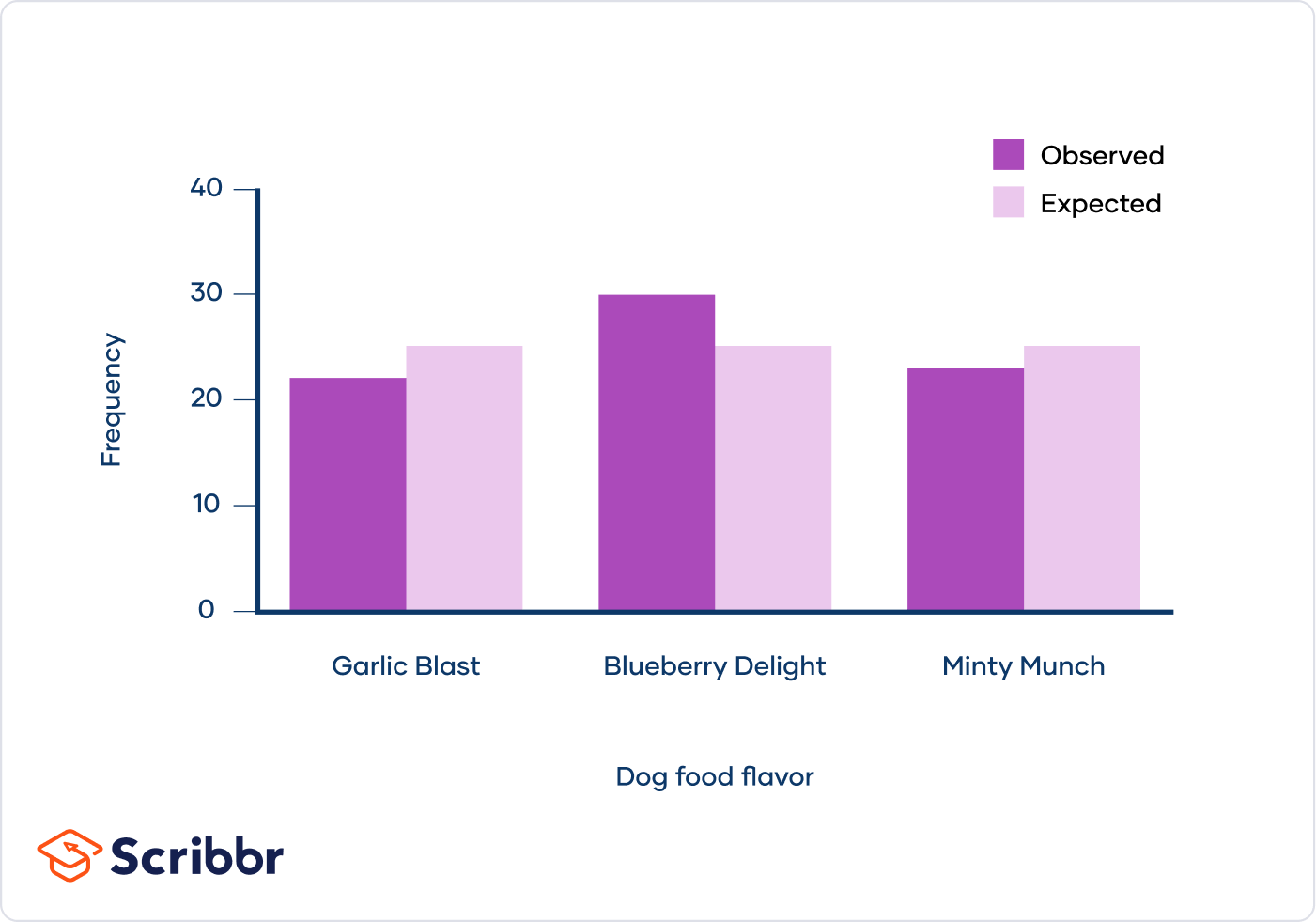
Example:
If a shop owner expects an equal number of customers each day over a week (7 days), and 210 customers visited the shop in total:
Expected Frequency per day = \( \frac{1}{7} \times 210 = 30 \)
2. For Chi-Square Test of Independence
The Chi-Square Test of Independence assesses whether two categorical variables are independent by comparing the observed frequencies in each category to the expected frequencies, assuming independence. To calculate the expected frequencies:
- Create a contingency table with observed frequencies.
- Compute the row and column totals for the table.
- Calculate the overall total of all observations.
- Use the formula to find the expected frequency for each cell:
Expected Frequency = \( \frac{(\text{Row Total}) \times (\text{Column Total})}{\text{Grand Total}} \)
Example:
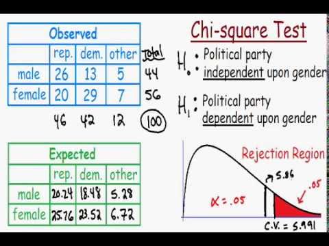
Consider a survey of 500 voters categorized by gender and political preference:
| Republican | Democrat | Independent | Total | |
| Male | 138 | 83 | 64 | 285 |
| Female | 64 | 67 | 84 | 215 |
| Total | 202 | 150 | 148 | 500 |
To find the expected frequency for Male Republicans:
Expected Frequency = \( \frac{(285 \times 202)}{500} = 115.14 \)
By repeating this calculation for each cell, you can fill in the expected frequencies for the entire contingency table.
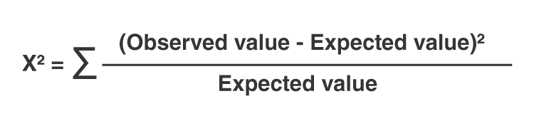
Chi-Square Test Statistic Formula
The chi-square test statistic is used to assess whether there is a significant difference between the expected and observed frequencies in one or more categories. The formula for the chi-square test statistic is:
\[ \chi^2 = \sum \frac{(O - E)^2}{E} \]
where:
- \(\chi^2\) is the chi-square test statistic
- \(O\) is the observed frequency
- \(E\) is the expected frequency
- \(\sum\) denotes the sum over all categories
To calculate the chi-square test statistic, follow these steps:
- Calculate the expected frequencies for each category using the formula: \[ E = \frac{(\text{row total} \times \text{column total})}{\text{grand total}} \]
- Compute the difference between the observed and expected frequencies for each category.
- Square the differences obtained in step 2.
- Divide the squared differences by the expected frequency for each category.
- Sum all the values obtained in step 4 to get the chi-square test statistic.
Here is a sample calculation:
| Category | Observed (O) | Expected (E) | (O - E) | (O - E)2 | (O - E)2 / E |
|---|---|---|---|---|---|
| Category 1 | 90 | 85 | 5 | 25 | 0.2941 |
| Category 2 | 60 | 55 | 5 | 25 | 0.4545 |
| Category 3 | 50 | 60 | -10 | 100 | 1.6667 |
Summing the values in the last column, we get the chi-square test statistic:
\[ \chi^2 = 0.2941 + 0.4545 + 1.6667 = 2.4153 \]
Once the chi-square statistic is calculated, it can be compared to a critical value from the chi-square distribution table based on the desired significance level and the degrees of freedom. The degrees of freedom for a chi-square test is calculated as:
\[ \text{df} = (r - 1) \times (c - 1) \]
where \( r \) is the number of rows and \( c \) is the number of columns in the contingency table. If the chi-square statistic is greater than the critical value, we reject the null hypothesis.
Degrees of Freedom in Chi-Square Test
Degrees of freedom (df) in a chi-square test are crucial as they affect the shape of the chi-square distribution and are used to determine the critical value needed to assess the statistical significance of the test result.
In a chi-square test, the degrees of freedom are calculated based on the number of categories or levels in the variables being analyzed. The general formulas for degrees of freedom in different types of chi-square tests are as follows:
- Chi-Square Test of Independence:
- This test is used to determine if there is a significant association between two categorical variables.
- The degrees of freedom are calculated using the formula:
\[
df = (r - 1) \times (c - 1)
\]
where \( r \) is the number of rows and \( c \) is the number of columns in the contingency table.
- Chi-Square Goodness of Fit Test:
- This test is used to determine if the observed frequencies in a single categorical variable match the expected frequencies based on a specific hypothesis.
- The degrees of freedom are calculated using the formula:
\[
df = k - 1
\]
where \( k \) is the number of categories or levels of the variable.
Let's look at an example for each type of test:
Example: Chi-Square Test of Independence
Suppose we want to test if there is a relationship between gender (male, female) and preference for a new product (like, dislike). The contingency table has 2 rows (genders) and 2 columns (preferences).
The degrees of freedom are calculated as:
\[
df = (2 - 1) \times (2 - 1) = 1
\]
Example: Chi-Square Goodness of Fit Test
Suppose we have a die and we want to test if it is fair. The die has 6 faces, so there are 6 categories.
The degrees of freedom are calculated as:
\[
df = 6 - 1 = 5
\]
Understanding and correctly calculating the degrees of freedom is essential for accurately interpreting the results of a chi-square test and determining whether the null hypothesis should be rejected.
Interpreting Chi-Square Test Results
The interpretation of Chi-Square test results involves several key steps to determine the significance and implications of the findings. Here is a detailed guide to help you interpret these results effectively:
-
Step 1: Determine the P-Value
The first step in interpreting the Chi-Square test results is to look at the p-value. The p-value indicates the probability that the observed differences (or greater) could occur under the null hypothesis. Compare the p-value to your significance level (commonly α = 0.05).
P \leq \alpha: The result is statistically significant. You reject the null hypothesis, indicating that there is an association between the variables.P > \alpha: The result is not statistically significant. You fail to reject the null hypothesis, indicating insufficient evidence to suggest an association between the variables.
-
Step 2: Examine the Test Statistic
The Chi-Square test statistic provides a measure of how much the observed frequencies deviate from the expected frequencies. A larger test statistic indicates a greater deviation from the expected frequencies under the null hypothesis.
-
Step 3: Review the Degrees of Freedom
The degrees of freedom (df) for a Chi-Square test depend on the number of categories in the variables being tested. It is calculated as:
df = (r - 1) \times (c - 1) where r is the number of rows and c is the number of columns in the contingency table. The degrees of freedom affect the critical value against which the test statistic is compared.
-
Step 4: Compare Observed and Expected Counts
Examine the observed and expected counts to identify which cells contribute most to the Chi-Square statistic. Large differences between observed and expected counts suggest stronger evidence against the null hypothesis.
Category Observed Count Expected Count Contribution to Chi-Square Category 1 O1 E1 (O1 - E1)² / E1 Category 2 O2 E2 (O2 - E2)² / E2 -
Step 5: Draw Conclusions
Based on the p-value and the comparison of observed and expected counts, draw conclusions about the association between the variables. If the p-value is below the significance level, conclude that there is a statistically significant association between the variables. If not, conclude that there is no sufficient evidence to suggest an association.
By following these steps, you can effectively interpret the results of a Chi-Square test and understand the implications of your statistical analysis.
Chi-Square Test of Independence
The Chi-Square Test of Independence is used to determine if there is a significant association between two categorical variables. This test is applicable when you have data organized in a contingency table where the rows represent categories of one variable and the columns represent categories of the other variable.
Steps to Perform the Chi-Square Test of Independence
- Formulate Hypotheses
- Null Hypothesis (\(H_0\)): There is no association between the two variables.
- Alternative Hypothesis (\(H_a\)): There is an association between the two variables.
- Calculate Expected Frequencies
For each cell in the contingency table, the expected frequency (\(E\)) is calculated using the formula:
\[
E_{ij} = \frac{( \text{Row Total}_i \times \text{Column Total}_j )}{\text{Grand Total}}
\] - Compute the Chi-Square Test Statistic
The Chi-Square statistic (\(\chi^2\)) is calculated as follows:
\[
\chi^2 = \sum \frac{(O_{ij} - E_{ij})^2}{E_{ij}}
\]where \(O_{ij}\) is the observed frequency and \(E_{ij}\) is the expected frequency.
- Determine Degrees of Freedom
The degrees of freedom (df) for the test are determined by the formula:
\[
\text{df} = (r - 1) \times (c - 1)
\]where \(r\) is the number of rows and \(c\) is the number of columns.
- Compare to Critical Value
Compare the calculated \(\chi^2\) value to the critical value from the Chi-Square distribution table at the desired significance level (commonly 0.05) and the calculated degrees of freedom.
- Make a Decision
If the calculated \(\chi^2\) value is greater than the critical value, reject the null hypothesis. Otherwise, fail to reject the null hypothesis.
- Interpret the Results
If you reject the null hypothesis, you conclude that there is a significant association between the two variables. If you fail to reject the null hypothesis, you conclude that there is no significant association between the two variables.
Example
Consider a study investigating the relationship between political affiliation (Democrat, Republican) and support for a tax reform bill (Support, Oppose, Indifferent). The data is collected from a sample of 500 individuals and organized in a 2x3 contingency table.
| Political Affiliation | Support | Oppose | Indifferent |
|---|---|---|---|
| Democrat | 138 | 83 | 64 |
| Republican | 64 | 67 | 84 |
Following the steps outlined above, you calculate the expected frequencies, the \(\chi^2\) statistic, and the degrees of freedom. After comparing the \(\chi^2\) value to the critical value, you can determine whether to reject the null hypothesis and conclude if there is an association between political affiliation and support for the tax reform bill.

Chi-Square Goodness of Fit Test
The Chi-Square Goodness of Fit Test is used to determine whether a sample data matches a population with a specific distribution. This test is applicable when you have one categorical variable from a single population. The main steps involved in conducting this test are:
- State the Hypotheses:
- Null Hypothesis (\(H_0\)): The data follows the specified distribution.
- Alternative Hypothesis (\(H_a\)): The data does not follow the specified distribution.
- Collect and Summarize Data:
- Collect observed frequencies for each category.
- Determine expected frequencies based on the hypothesized distribution.
- Calculate the Test Statistic:
The test statistic for the Chi-Square Goodness of Fit Test is calculated using the formula:
\[
\chi^2 = \sum \frac{(O_i - E_i)^2}{E_i}
\]where \(O_i\) is the observed frequency and \(E_i\) is the expected frequency for category \(i\).
- Determine Degrees of Freedom:
Degrees of freedom for this test is calculated as:
\[
df = k - 1
\]where \(k\) is the number of categories.
- Compare to Critical Value:
Compare the calculated \(\chi^2\) statistic to the critical value from the Chi-Square distribution table at the desired significance level (\(\alpha\)).
- If \(\chi^2\) statistic > critical value, reject the null hypothesis.
- If \(\chi^2\) statistic ≤ critical value, do not reject the null hypothesis.
The Chi-Square Goodness of Fit Test helps in understanding whether the observed sample distribution deviates significantly from the expected distribution, providing insights into the consistency of data with theoretical expectations.
Assumptions of Chi-Square Test
The Chi-Square test is a widely used statistical method, but its validity depends on certain assumptions being met. Here are the key assumptions of the Chi-Square test:
- Independence of Observations: Each observation should be independent of the others. This means that the occurrence of one event does not affect the occurrence of another.
- Mutually Exclusive Categories: The data should be categorized into mutually exclusive categories. Each observation should fit into one and only one category in the contingency table.
- Sufficient Sample Size: The expected frequency in each cell of the contingency table should be at least 5. Specifically, at least 80% of the expected frequencies should be 5 or more, and no cell should have an expected frequency less than 1.
- Count Data: The Chi-Square test is appropriate for frequency data or count data, not for continuous data unless they are categorized.
These assumptions ensure the reliability of the Chi-Square test results. If these assumptions are violated, the test may not produce valid results, and alternative statistical tests or data modifications may be necessary.
Examples of Chi-Square Test Applications
The Chi-Square test is widely used in various fields to test the independence of categorical variables or the goodness of fit. Here are some examples of its applications:
1. Chi-Square Test of Independence
This test determines whether there is a significant association between two categorical variables. It is commonly used in research fields such as sociology, marketing, and biology.
- Sociology: Examining the relationship between gender and voting preference in an election.
- Marketing: Assessing whether the choice of a product is independent of the region where it is sold.
- Biology: Determining if there is a link between a genetic trait and the presence of a certain disease.
2. Chi-Square Goodness of Fit Test
This test is used to determine if a sample data matches a population with a specific distribution. It is particularly useful in fields like quality control and genetics.
- Quality Control: Checking if the number of defective products follows a particular distribution pattern.
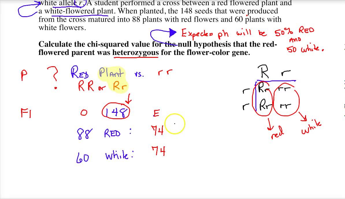
- Genetics: Testing if the observed frequencies of different phenotypes in a population match the expected ratios based on Mendelian inheritance.
Example Calculation: Recycling Intervention Study
Consider a study examining the effectiveness of different interventions to encourage recycling. The observed and expected frequencies of households that recycle or do not recycle after receiving different types of interventions (flyer, phone call, control) are analyzed.
| Intervention | Outcome | Observed (O) | Expected (E) | (O - E) | (O - E)^2 | (O - E)^2 / E |
|---|---|---|---|---|---|---|
| Flyer | Recycle | 89 | 84.61 | 4.39 | 19.27 | 0.23 |
| Flyer | Not Recycle | 9 | 13.39 | -4.39 | 19.27 | 1.44 |
| Phone Call | Recycle | 84 | 79.43 | 4.57 | 20.88 | 0.26 |
| Phone Call | Not Recycle | 8 | 12.57 | -4.57 | 20.88 | 1.66 |
| Control | Recycle | 86 | 94.97 | -8.97 | 80.46 | 0.85 |
| Control | Not Recycle | 24 | 15.03 | 8.97 | 80.46 | 5.35 |
| Chi-Square Statistic | 9.79 | |||||
The Chi-Square statistic is 9.79. By comparing this to a critical value from the Chi-Square distribution table, one can determine whether to reject the null hypothesis that the interventions are equally effective in promoting recycling.
Common Mistakes and How to Avoid Them
When conducting a Chi-Square test, several common mistakes can affect the validity and reliability of your results. Here are some of the most frequent errors and how to avoid them:
- Using Inappropriate Data Types
Chi-Square tests are designed for categorical data, not continuous or ordinal data. Ensure that your data is nominal before applying the test.
- Ignoring the Assumptions of the Test
One key assumption is that the expected frequency in each cell should be at least 5. If this condition is not met, consider combining categories or using a different test, such as Fisher's Exact Test.
- Misinterpreting Causality
A significant Chi-Square test indicates an association between variables, not causation. Avoid making causal inferences based solely on Chi-Square results.
- Incorrectly Calculating Expected Frequencies
Ensure that you accurately calculate the expected frequencies based on the marginal totals and the overall sample size. Mistakes in this step can lead to incorrect conclusions.
- Overlooking the Effect Size
Even if your test is significant, the effect size (e.g., Cramer's V or Phi coefficient) should be calculated to understand the strength of the association. This is especially important in large samples where small differences can be statistically significant.
- Ignoring the Sample Size
Chi-Square tests can be unreliable with small sample sizes. Ensure that your sample is large enough to provide reliable results, or consider using an alternative statistical method.
- Failing to Report the Degrees of Freedom
Always report the degrees of freedom along with the Chi-Square statistic and p-value. This provides essential context for interpreting the test results.
- Misunderstanding the Null Hypothesis
The null hypothesis in a Chi-Square test states that there is no association between the variables. Ensure that you correctly interpret what rejecting or failing to reject the null hypothesis implies for your research.
- Not Checking for Data Entry Errors
Data entry mistakes can skew your results. Double-check your data before performing the test to ensure accuracy.
By being aware of these common mistakes and taking steps to avoid them, you can ensure that your Chi-Square test results are valid and reliable.
Advantages and Limitations of Chi-Square Test
The Chi-Square test is a powerful statistical tool used to determine if there is a significant association between categorical variables. Here, we outline the key advantages and limitations of this test.
Advantages
- Simplicity: The Chi-Square test is straightforward to calculate and interpret, making it accessible for researchers and analysts with basic statistical knowledge.
- Applicability: It can be used for a variety of applications, including testing the independence of two categorical variables and assessing the goodness of fit between observed and expected frequencies.
- Non-parametric nature: Since the Chi-Square test is non-parametric, it does not assume a normal distribution of the data, allowing it to be used with nominal data and ordinal data.
- Wide usage: It is extensively used in fields like social sciences, marketing, and medical research to analyze survey data and observational studies.
- Flexibility: The test can handle large datasets and multiple categories, providing robust insights into complex relationships.
Limitations
- Sample size dependency: The Chi-Square test requires a sufficiently large sample size to ensure reliable results. Small sample sizes may lead to inaccurate conclusions.
- Expected frequency constraints: For the test to be valid, the expected frequency in each category should be at least 5. Categories with smaller expected frequencies may distort the test results.
- Insensitive to small differences: The test may not detect small but potentially important differences between observed and expected frequencies, especially in large samples.
- Assumes independence: The Chi-Square test assumes that the observations are independent of each other. Violations of this assumption can lead to misleading results.
- Limited to categorical data: It is only applicable to categorical data and cannot be used for continuous data without converting it into categorical form, which may result in loss of information.
By understanding these advantages and limitations, researchers can effectively use the Chi-Square test to draw meaningful conclusions from categorical data, while being mindful of its constraints.
Kiểm Tra Chi-Square
READ MORE:
Thống kê Chi-Square cho kiểm định giả thuyết | AP Statistics | Khan Academy
:max_bytes(150000):strip_icc()/Chi-SquareStatistic_Final_4199464-7eebcd71a4bf4d9ca1a88d278845e674.jpg)