Topic x squared divided by 2: Discover the fascinating world of the mathematical expression \( \frac{x^2}{2} \). This comprehensive guide delves into its properties, graphical representation, and wide-ranging applications in fields like physics and economics. Whether you're a student or an enthusiast, learn how this fundamental concept can enhance your understanding of mathematics.
Table of Content
- Understanding the Expression: \( \frac{x^2}{2} \)
- Introduction to Quadratic Functions
- Understanding \( \frac{x^2}{2} \)
- Graphical Representation of \( \frac{x^2}{2} \)
- Key Features and Properties
- Applications in Mathematics
- Applications in Physics
- Applications in Economics
- Calculating Derivatives
- Calculating Integrals
- Solving Equations Involving \( \frac{x^2}{2} \)
- Optimization Problems
- Real-World Examples
- YOUTUBE: Video này giải thích làm thế nào để tìm số mà khi bình phương chia cho 2 thì bằng 50.
Understanding the Expression: \( \frac{x^2}{2} \)
The expression \( \frac{x^2}{2} \) represents a quadratic function divided by a constant. This form is common in various mathematical applications, including calculus, physics, and engineering.
Key Features
- Quadratic Function: The term \( x^2 \) indicates that the function is quadratic, which means it creates a parabola when graphed.
- Division by Constant: Dividing by 2 scales the function, making it "wider" compared to the standard \( x^2 \) function.
Graphical Representation
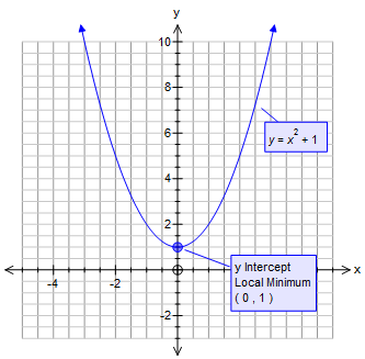
When graphing \( \frac{x^2}{2} \), the parabola opens upwards, and its vertex is at the origin (0, 0). The function is symmetric around the y-axis.
Here is the general shape of the graph:
Derivative
The derivative of \( \frac{x^2}{2} \) with respect to x is found using the power rule:
\[
\frac{d}{dx}\left(\frac{x^2}{2}\right) = x
\]
This derivative indicates the slope of the tangent to the curve at any point x.
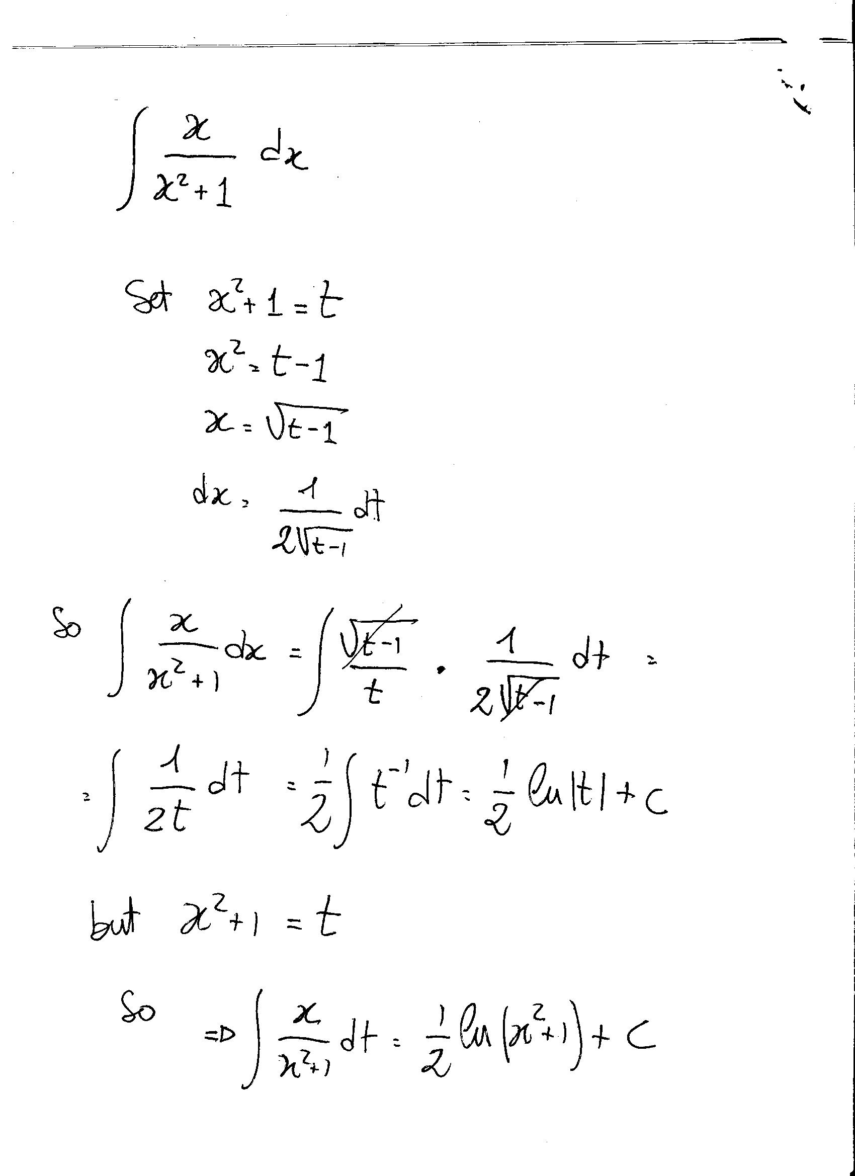
Integral
The integral of \( \frac{x^2}{2} \) with respect to x is computed as follows:
\[
\int \frac{x^2}{2} \, dx = \frac{x^3}{6} + C
\]
Here, C represents the constant of integration.
Applications
This function appears in various contexts, such as:
- Physics: Describing potential energy in a quadratic potential field.
- Economics: Modeling cost functions where costs increase quadratically with production levels.
- Mathematics: Solving differential equations and optimization problems.
Conclusion
The expression \( \frac{x^2}{2} \) is a fundamental mathematical function with significant applications in multiple fields. Understanding its properties, including its graph, derivative, and integral, is essential for various practical and theoretical purposes.
READ MORE:
Introduction to Quadratic Functions
Quadratic functions are fundamental in algebra and appear in various forms across mathematics and its applications. A quadratic function is any function that can be written in the form:
\[
f(x) = ax^2 + bx + c
\]
where \( a \), \( b \), and \( c \) are constants, and \( a \neq 0 \).
The standard form of a quadratic function highlights its key characteristics:
- Parabolic Shape: The graph of a quadratic function is a parabola, which can open upwards or downwards depending on the sign of \( a \).
- Vertex: The highest or lowest point on the parabola, known as the vertex, is given by the formula \(\left( -\frac{b}{2a}, f\left(-\frac{b}{2a}\right) \right)\).
- Axis of Symmetry: The vertical line that passes through the vertex and divides the parabola into two symmetric halves is \( x = -\frac{b}{2a} \).
- Roots or Zeros: The solutions to the equation \( ax^2 + bx + c = 0 \), found using the quadratic formula \[ x = \frac{-b \pm \sqrt{b^2 - 4ac}}{2a} \], represent the points where the parabola intersects the x-axis.
Quadratic functions are versatile and have numerous applications in various fields. For instance, they are used to model projectile motion in physics, determine profit maximization in economics, and solve optimization problems in calculus.
An example of a specific quadratic function is \( \frac{x^2}{2} \), which simplifies the general form by setting \( a = \frac{1}{2} \), \( b = 0 \), and \( c = 0 \). This particular function will be explored in more detail in the following sections.
Understanding \( \frac{x^2}{2} \)
The expression \( \frac{x^2}{2} \) represents a simple yet important quadratic function in mathematics. It is a special case of the general quadratic function \( ax^2 + bx + c \) where \( a = \frac{1}{2} \), \( b = 0 \), and \( c = 0 \).
To understand this function better, let's break it down into its key components:
- Coefficient: The coefficient \( \frac{1}{2} \) in front of \( x^2 \) means that for every unit increase in \( x \), the value of the function increases by half the square of that unit. This coefficient affects the "width" of the parabola, making it wider compared to the standard \( x^2 \) function.
- Vertex: Since the linear term and the constant term are both zero, the vertex of the parabola is at the origin, \((0, 0)\). This is the lowest point of the parabola since the coefficient of \( x^2 \) is positive.
- Symmetry: The function is symmetric about the y-axis. This is because changing \( x \) to \( -x \) does not change the value of \( \frac{x^2}{2} \).
To visualize the function \( \frac{x^2}{2} \), consider its graph:
The graph is a parabola that opens upwards with its vertex at the origin.
Let's look at the function through some specific examples:
- When \( x = 0 \), \( y = \frac{0^2}{2} = 0 \).
- When \( x = 1 \), \( y = \frac{1^2}{2} = \frac{1}{2} \).
- When \( x = 2 \), \( y = \frac{2^2}{2} = 2 \).
- When \( x = -2 \), \( y = \frac{(-2)^2}{2} = 2 \).
The derivative of \( \frac{x^2}{2} \) with respect to \( x \) is:
\[
\frac{d}{dx}\left(\frac{x^2}{2}\right) = x
\]
This represents the slope of the tangent line to the curve at any point \( x \).
The integral of \( \frac{x^2}{2} \) with respect to \( x \) is:
\[
\int \frac{x^2}{2} \, dx = \frac{x^3}{6} + C
\]
where \( C \) is the constant of integration.
Understanding \( \frac{x^2}{2} \) provides a foundation for exploring more complex quadratic functions and their applications in various fields such as physics, economics, and engineering. It illustrates how changing coefficients and terms in a quadratic function affects its graph and properties.
Graphical Representation of \( \frac{x^2}{2} \)
The function \( \frac{x^2}{2} \) represents a parabola, a common and significant shape in mathematics. Understanding its graphical representation helps to visualize its properties and behavior.
Here are the key steps to graph \( \frac{x^2}{2} \):
- Identify the Vertex: The vertex of the parabola is at the origin, \((0, 0)\). This is because there are no linear or constant terms to shift the vertex from the origin.
- Determine the Direction: Since the coefficient of \( x^2 \) is positive (\( \frac{1}{2} \)), the parabola opens upwards.
- Calculate Key Points: Select a few values of \( x \) to find corresponding values of \( y \). For example:
- When \( x = -2 \), \( y = \frac{(-2)^2}{2} = 2 \)
- When \( x = -1 \), \( y = \frac{(-1)^2}{2} = 0.5 \)
- When \( x = 0 \), \( y = \frac{0^2}{2} = 0 \)
- When \( x = 1 \), \( y = \frac{1^2}{2} = 0.5 \)
- When \( x = 2 \), \( y = \frac{2^2}{2} = 2 \)
- Plot the Points: Using the calculated points, plot them on a coordinate plane:
x y -2 2 -1 0.5 0 0 1 0.5 2 2 - Draw the Parabola: Connect the points smoothly to form the parabola. The graph will be symmetric about the y-axis.
The resulting graph of \( \frac{x^2}{2} \) is a parabola that opens upwards with its vertex at the origin:
Properties of the Graph:
- Symmetry: The parabola is symmetric about the y-axis. This means for any point \((x, y)\) on the graph, there is a corresponding point \((-x, y)\).
- Vertex: The lowest point on the graph is the vertex at \((0, 0)\).
- Opening Direction: Since the coefficient of \( x^2 \) is positive, the parabola opens upwards.
- Width: The coefficient \( \frac{1}{2} \) makes the parabola wider than the standard \( x^2 \) parabola. A smaller coefficient makes the parabola wider, while a larger coefficient makes it narrower.
Understanding the graphical representation of \( \frac{x^2}{2} \) is essential for analyzing its behavior and applying it to real-world situations. The graph provides a visual insight into how the function changes with different values of \( x \).
Key Features and Properties
The expression \( \frac{x^2}{2} \) possesses several key features and properties that are essential to understanding its behavior and applications in various fields. Below, we explore these features in detail:
- Form: The function \( \frac{x^2}{2} \) is a quadratic function, which can be written in the general form \( ax^2 + bx + c \) with \( a = \frac{1}{2} \), \( b = 0 \), and \( c = 0 \).
- Vertex: The vertex of the function is at the origin, \((0, 0)\). This is the lowest point on the graph since the parabola opens upwards.
- Axis of Symmetry: The axis of symmetry for the function is the y-axis, or \( x = 0 \). This means the graph is symmetric around this vertical line.
- Direction of Opening: The parabola opens upwards because the coefficient of \( x^2 \) is positive. If the coefficient were negative, the parabola would open downwards.
- Width: The coefficient \( \frac{1}{2} \) makes the parabola wider than the standard parabola \( y = x^2 \). A smaller coefficient (in absolute value) results in a wider parabola, while a larger coefficient makes it narrower.
- Intercepts:
- Y-intercept: The y-intercept is the point where the graph intersects the y-axis. For \( \frac{x^2}{2} \), this occurs at \((0, 0)\).
- X-intercepts: The x-intercepts are the points where the graph intersects the x-axis. For \( \frac{x^2}{2} \), this also occurs at \((0, 0)\). Since the vertex is at the origin and the parabola opens upwards, there are no other x-intercepts.
- End Behavior: As \( x \) approaches positive or negative infinity, \( y \) approaches positive infinity. This is typical for parabolas that open upwards.
- Rate of Change: The derivative of \( \frac{x^2}{2} \) with respect to \( x \) is \( x \), indicating that the rate of change increases linearly as \( x \) increases. This means the slope of the tangent line to the graph becomes steeper as \( x \) moves away from the origin.
\[
\frac{d}{dx}\left(\frac{x^2}{2}\right) = x
\] - Area Under the Curve: The integral of \( \frac{x^2}{2} \) with respect to \( x \) gives the area under the curve from a point to the origin. This is useful for applications in physics and engineering where the area represents accumulated quantities.
\[
\int \frac{x^2}{2} \, dx = \frac{x^3}{6} + C
\]
Understanding these key features and properties of \( \frac{x^2}{2} \) provides a comprehensive view of how the function behaves and how it can be applied in different mathematical and practical contexts.
Applications in Mathematics
The function \( \frac{x^2}{2} \) plays a significant role in various mathematical contexts, offering insights and solutions across different areas of study. Below are some key applications:
- Calculus:
- Derivatives: The derivative of \( \frac{x^2}{2} \) is \( x \), which helps in understanding the rate of change and slope of the tangent at any point on the curve.
\[
\frac{d}{dx}\left(\frac{x^2}{2}\right) = x
\] - Integrals: The integral of \( \frac{x^2}{2} \) is used to find the area under the curve, which is crucial in various applications such as finding displacement from velocity.
\[
\int \frac{x^2}{2} \, dx = \frac{x^3}{6} + C
\]
- Derivatives: The derivative of \( \frac{x^2}{2} \) is \( x \), which helps in understanding the rate of change and slope of the tangent at any point on the curve.
- Algebra:
- Solving Quadratic Equations: The function helps in solving quadratic equations of the form \( ax^2 + bx + c = 0 \), particularly when \( a = \frac{1}{2} \), \( b = 0 \), and \( c = 0 \).
- Graphical Analysis: Understanding the graph of \( \frac{x^2}{2} \) aids in analyzing and interpreting other quadratic functions by comparing their shapes and transformations.
- Optimization Problems: The function is used in optimization problems where finding the minimum or maximum values of quadratic functions is required. For \( \frac{x^2}{2} \), the minimum value occurs at the vertex \((0, 0)\).
- Physics and Engineering: In physics, \( \frac{x^2}{2} \) can represent potential energy in a quadratic potential field. In engineering, it is used to model various systems and phenomena where quadratic relationships are present.
- Mathematical Modeling: The function \( \frac{x^2}{2} \) is employed in creating mathematical models that describe real-world phenomena, particularly those involving acceleration, force, and energy relationships.
These applications illustrate the versatility and importance of the function \( \frac{x^2}{2} \) in mathematics, providing foundational knowledge and tools for solving a wide range of problems.
Applications in Physics
The function \( \frac{x^2}{2} \) finds numerous applications in physics, playing a crucial role in understanding various physical phenomena and solving problems. Below are some key applications:
- Kinematics:
- Displacement: In uniformly accelerated motion, the displacement \( s \) can be expressed as a quadratic function of time \( t \), where \( s = \frac{1}{2} a t^2 \). Here, \( a \) is the constant acceleration, making the displacement a direct application of \( \frac{x^2}{2} \).
- Position-Time Graphs: The position of an object under constant acceleration is often represented by a parabola. The function \( \frac{x^2}{2} \) helps in analyzing the object's motion over time.
- Potential Energy:
- Harmonic Oscillators: The potential energy \( U \) of a harmonic oscillator (e.g., a mass-spring system) is given by \( U = \frac{1}{2} k x^2 \), where \( k \) is the spring constant and \( x \) is the displacement from equilibrium. This is a direct application of the \( \frac{x^2}{2} \) form.
- Gravitational Potential Energy: For small displacements in a gravitational field, the potential energy can sometimes be approximated by a quadratic function, aiding in the analysis of oscillatory motion.
- Electric Fields:
- Energy Stored in Capacitors: The energy \( U \) stored in a capacitor is given by \( U = \frac{1}{2} C V^2 \), where \( C \) is the capacitance and \( V \) is the voltage. This quadratic relationship is crucial in circuit analysis and design.
- Projectile Motion:
- Trajectory Analysis: The vertical displacement of a projectile under the influence of gravity is a quadratic function of time, described by \( y = y_0 + v_0 t - \frac{1}{2} g t^2 \), where \( g \) is the acceleration due to gravity. Understanding the function \( \frac{x^2}{2} \) helps in analyzing projectile paths.
- Mechanics:
- Work-Energy Theorem: The work done by a variable force can be determined using the integral of a quadratic function. For example, the work done by a spring force \( F = -kx \) over a displacement \( x \) involves integrating \( \frac{kx^2}{2} \).
These applications illustrate the importance of \( \frac{x^2}{2} \) in physics, providing a foundation for understanding and solving complex physical problems.
Applications in Economics
The function \( \frac{x^2}{2} \) can be utilized in various economic models and analyses to represent costs, revenue, and other economic factors. Below are some key applications:
- Cost Functions:
- Total Cost: In microeconomics, the total cost (TC) of producing goods can sometimes be modeled as a quadratic function of the quantity produced (Q). For instance, a simple cost function might be \( TC = \frac{1}{2} Q^2 \), where costs increase quadratically with the quantity of output.
- Marginal Cost: The marginal cost (MC), or the cost of producing one additional unit, is the derivative of the total cost function. For \( TC = \frac{1}{2} Q^2 \), the marginal cost is \( MC = Q \), showing a linear relationship between quantity and cost.
\[
\frac{d}{dQ}\left(\frac{Q^2}{2}\right) = Q
\]
- Revenue Functions:
- Total Revenue: Similar to cost functions, total revenue (TR) can also be modeled using quadratic functions. For example, if the price decreases linearly with quantity due to demand constraints, total revenue might be modeled as \( TR = PQ = (P_0 - bQ)Q = P_0Q - bQ^2 \), where \( P_0 \) is the initial price and \( b \) is the rate of decrease in price.
- Profit Maximization:
- Profit Function: The profit (\(\Pi\)) is the difference between total revenue and total cost. If both are quadratic functions, the resulting profit function may also be quadratic. For instance, if \( TR = P_0Q - bQ^2 \) and \( TC = \frac{1}{2} Q^2 \), then \( \Pi = TR - TC = P_0Q - bQ^2 - \frac{1}{2} Q^2 \).
- Optimal Output: To find the quantity that maximizes profit, set the derivative of the profit function with respect to \( Q \) to zero and solve for \( Q \). This involves quadratic optimization techniques commonly used in economics.
\[
\frac{d}{dQ}\left(P_0Q - bQ^2 - \frac{1}{2}Q^2\right) = P_0 - 2bQ - Q = 0
\]
- Utility Functions:
- Quadratic Utility: In some economic models, utility functions are expressed as quadratic functions of consumption. For instance, a utility function \( U(x) = \frac{x^2}{2} \) indicates diminishing marginal utility, where the additional satisfaction from consuming an extra unit decreases as consumption increases.
These applications demonstrate the versatility of the function \( \frac{x^2}{2} \) in economic theory and practice, aiding in the analysis and optimization of various economic phenomena.
Calculating Derivatives
The derivative of a function provides information about its rate of change. In this section, we will calculate the derivative of the function \( \frac{x^2}{2} \) and discuss its significance.
Step-by-Step Calculation
Start with the function:
\[ f(x) = \frac{x^2}{2} \]
Recall the power rule for differentiation:
\[ \frac{d}{dx} \left( x^n \right) = nx^{n-1} \]
Apply the power rule to \( x^2 \):
\[ \frac{d}{dx} \left( x^2 \right) = 2x \]
Since the function is \( \frac{x^2}{2} \), multiply the result by \( \frac{1}{2} \):
\[ \frac{d}{dx} \left( \frac{x^2}{2} \right) = \frac{1}{2} \cdot 2x = x \]
Result
The derivative of the function \( \frac{x^2}{2} \) is:
\[ \frac{d}{dx} \left( \frac{x^2}{2} \right) = x \]
Interpretation
The derivative \( x \) represents the slope of the function \( \frac{x^2}{2} \) at any given point \( x \). This means:
- For \( x > 0 \), the slope is positive, indicating an increasing function.
- For \( x < 0 \), the slope is negative, indicating a decreasing function.
- At \( x = 0 \), the slope is zero, corresponding to a local minimum.
Graphical Representation
Graphically, the derivative \( x \) can be represented as the tangent line's slope at any point on the curve of \( \frac{x^2}{2} \).
Below is a table summarizing the derivative at various points:
| x | \( f(x) = \frac{x^2}{2} \) | \( f'(x) \) |
|---|---|---|
| -2 | 2 | -2 |
| -1 | 0.5 | -1 |
| 0 | 0 | 0 |
| 1 | 0.5 | 1 |
| 2 | 2 | 2 |
Calculating Integrals
Integration is the process of finding the antiderivative of a function. In this section, we will calculate the integral of the function \( \frac{x^2}{2} \) and interpret its result.
Step-by-Step Calculation
Start with the function to be integrated:
\[ f(x) = \frac{x^2}{2} \]
Recall the power rule for integration:
\[ \int x^n \, dx = \frac{x^{n+1}}{n+1} + C \]
Apply the power rule to \( x^2 \):
\[ \int x^2 \, dx = \frac{x^3}{3} + C \]
Since the function is \( \frac{x^2}{2} \), include the constant factor \( \frac{1}{2} \):
\[ \int \frac{x^2}{2} \, dx = \frac{1}{2} \int x^2 \, dx = \frac{1}{2} \cdot \frac{x^3}{3} + C = \frac{x^3}{6} + C \]
Result
The integral of the function \( \frac{x^2}{2} \) is:
\[ \int \frac{x^2}{2} \, dx = \frac{x^3}{6} + C \]
Interpretation
The antiderivative \( \frac{x^3}{6} + C \) represents a family of functions whose derivative is \( \frac{x^2}{2} \). The constant \( C \) is an arbitrary constant that accounts for the indefinite nature of the integral.
Definite Integral
To compute the definite integral of \( \frac{x^2}{2} \) over an interval \([a, b]\), evaluate the antiderivative at the bounds and subtract:
\[ \int_a^b \frac{x^2}{2} \, dx = \left[ \frac{x^3}{6} \right]_a^b = \frac{b^3}{6} - \frac{a^3}{6} \]
Graphical Representation
Graphically, the integral of \( \frac{x^2}{2} \) over an interval \([a, b]\) represents the area under the curve from \( x = a \) to \( x = b \).
Below is a table summarizing the integral over various intervals:
| Interval \([a, b]\) | Definite Integral \(\int_a^b \frac{x^2}{2} \, dx\) |
|---|---|
| \([0, 1]\) | \(\frac{1}{6}\) |
| \([0, 2]\) | \(\frac{8}{6} = \frac{4}{3}\) |
| \([1, 2]\) | \(\frac{8}{6} - \frac{1}{6} = \frac{7}{6}\) |
| \([1, 3]\) | \(\frac{27}{6} - \frac{1}{6} = \frac{26}{6} = \frac{13}{3}\) |
Solving Equations Involving \( \frac{x^2}{2} \)
Solving equations involving the function \( \frac{x^2}{2} \) typically involves finding the value of \( x \) that satisfies the equation. We will explore different types of equations and provide step-by-step solutions.
Step-by-Step Solutions
1. Solving Simple Equations
Consider the equation:
\[ \frac{x^2}{2} = k \]
Multiply both sides by 2 to clear the fraction:
\[ x^2 = 2k \]
Take the square root of both sides to solve for \( x \):
\[ x = \pm \sqrt{2k} \]
Example
To solve \( \frac{x^2}{2} = 8 \):
Multiply by 2:
\[ x^2 = 16 \]
Take the square root:
\[ x = \pm 4 \]
Thus, the solutions are \( x = 4 \) and \( x = -4 \).
2. Solving Quadratic Equations
Consider the quadratic equation involving \( \frac{x^2}{2} \) and a linear term:
\[ \frac{x^2}{2} + bx + c = 0 \]
Multiply through by 2 to obtain a standard quadratic form:
\[ x^2 + 2bx + 2c = 0 \]
Use the quadratic formula:
\[ x = \frac{-2b \pm \sqrt{(2b)^2 - 4 \cdot 1 \cdot 2c}}{2 \cdot 1} = \frac{-2b \pm \sqrt{4b^2 - 8c}}{2} = \frac{-2b \pm 2\sqrt{b^2 - 2c}}{2} \]
\[ x = -b \pm \sqrt{b^2 - 2c} \]
Example
To solve \( \frac{x^2}{2} + 3x + 2 = 0 \):
Multiply by 2:
\[ x^2 + 6x + 4 = 0 \]
Apply the quadratic formula:
\[ x = \frac{-6 \pm \sqrt{6^2 - 4 \cdot 1 \cdot 4}}{2 \cdot 1} = \frac{-6 \pm \sqrt{36 - 16}}{2} = \frac{-6 \pm \sqrt{20}}{2} \]
\[ x = \frac{-6 \pm 2\sqrt{5}}{2} = -3 \pm \sqrt{5} \]
Thus, the solutions are \( x = -3 + \sqrt{5} \) and \( x = -3 - \sqrt{5} \).
3. Solving Equations with Constants
Consider an equation where \( \frac{x^2}{2} \) equals a constant \( k \):
\[ \frac{x^2}{2} = k \]
Multiply by 2:
\[ x^2 = 2k \]
Take the square root:
\[ x = \pm \sqrt{2k} \]
Example
To solve \( \frac{x^2}{2} = 10 \):
Multiply by 2:
\[ x^2 = 20 \]
Take the square root:
\[ x = \pm \sqrt{20} = \pm 2\sqrt{5} \]
Thus, the solutions are \( x = 2\sqrt{5} \) and \( x = -2\sqrt{5} \).
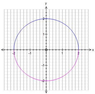
Graphical Representation
Graphically, the solutions represent the points where the curve \( \frac{x^2}{2} \) intersects with the horizontal line \( y = k \).
Summary
In summary, solving equations involving \( \frac{x^2}{2} \) can be approached by transforming the equation into a standard quadratic form, applying the quadratic formula, and interpreting the results.
Optimization Problems
Optimization problems involving the function \( \frac{x^2}{2} \) often require finding the maximum or minimum values of this function under certain constraints. Here, we will explore a step-by-step approach to solving such problems.
Example Problem
Consider the problem of finding the minimum value of \( \frac{x^2}{2} \) given a specific constraint. Let's solve this through a series of steps:
-
Define the Objective Function:
The objective function we want to minimize is:
\[
f(x) = \frac{x^2}{2}
\] -
Identify the Constraint:
Assume we have a constraint such as \( g(x) = x - c = 0 \), where \( c \) is a constant.
-
Set Up the Lagrangian:
To incorporate the constraint, we use the Lagrangian method. The Lagrangian function \( \mathcal{L} \) is given by:
\[
\mathcal{L}(x, \lambda) = \frac{x^2}{2} + \lambda (x - c)
\]where \( \lambda \) is the Lagrange multiplier.
-
Compute the Partial Derivatives:
Calculate the partial derivatives of \( \mathcal{L} \) with respect to \( x \) and \( \lambda \):
\[
\frac{\partial \mathcal{L}}{\partial x} = x + \lambda = 0
\]\[
\frac{\partial \mathcal{L}}{\partial \lambda} = x - c = 0
\] -
Solve the System of Equations:
Solve the equations obtained from the partial derivatives:
From \( \frac{\partial \mathcal{L}}{\partial x} = 0 \):
\[
x + \lambda = 0 \implies \lambda = -x
\]From \( \frac{\partial \mathcal{L}}{\partial \lambda} = 0 \):
\[
x - c = 0 \implies x = c
\] -
Find the Minimum Value:
Substitute \( x = c \) back into the objective function:
\[
f(c) = \frac{c^2}{2}
\]Thus, the minimum value of \( \frac{x^2}{2} \) given the constraint \( x = c \) is \( \frac{c^2}{2} \).
Applications
Optimization problems involving quadratic functions like \( \frac{x^2}{2} \) are common in various fields:
- Economics: Minimizing cost functions.
- Physics: Finding the point of equilibrium.
- Engineering: Optimizing design parameters for efficiency.
Conclusion
Optimization of \( \frac{x^2}{2} \) involves using techniques such as the Lagrangian method to find the function's minimum or maximum values under given constraints. These methods are widely applicable in diverse fields, making them crucial for problem-solving in mathematics and beyond.
Real-World Examples
Quadratic functions like \( \frac{x^2}{2} \) appear in various real-world contexts. Here are some notable examples:
Projectile Motion
One of the most common applications of quadratic functions is in the modeling of projectile motion. The height of an object thrown into the air follows a parabolic trajectory, which can be represented by a quadratic equation. For example, if a ball is thrown upwards, its height \( h \) at time \( t \) can be described by:
\[ h(t) = -5t^2 + 14t + 3 \]
Here, the term \( -5t^2 \) represents the effect of gravity, while the other terms account for the initial velocity and height. This quadratic function allows us to calculate key points such as the maximum height and the time the ball hits the ground.
Optimization in Business
Quadratic functions are also used in business to model and optimize profits. For example, consider a company that sells a product and incurs both fixed and variable costs. The profit function can be modeled as a quadratic equation. Suppose the profit \( P \) depends on the price \( x \) of the product:
\[ P(x) = -200x^2 + 92,000x - 8,400,000 \]
By finding the vertex of this parabola, we can determine the price that maximizes profit. In this case, solving the equation shows that the optimal price is $230, leading to maximum profit.
Structural Engineering
In structural engineering, quadratic functions help in designing frames and other structures. For instance, if a rectangular frame is to be cut out from a sheet of metal with certain constraints, the area of the frame can be described by a quadratic equation. Suppose we need a frame with an internal area of 28 cm² and dimensions of 11 cm by 6 cm, the width \( x \) of the metal border around the frame can be determined by:
\[ 4x^2 + 34x = 28 \]
Solving this equation gives the necessary width for the frame to meet the area requirement.
River Speed Problems
Quadratic equations can also be used to solve problems involving relative speeds, such as determining the speed of a boat traveling upstream and downstream in a river. If a boat travels a total distance of 15 km upstream and back downstream in 3 hours, and the river current is 2 km/h, we can set up the equation:
\[ 3(x^2 - 4) = 15x + 15(x-4) \]
Solving this quadratic equation helps find the boat's speed in still water and the time taken for each part of the journey.
These examples illustrate how quadratic functions, including \( \frac{x^2}{2} \), are essential in various practical applications, helping to solve problems and optimize outcomes in physics, business, engineering, and more.

READ MORE:
Video này giải thích làm thế nào để tìm số mà khi bình phương chia cho 2 thì bằng 50.
Một số bình phương chia cho 2 là 50, số đó là bao nhiêu?