Topic antiderivative of x squared: Discover the fundamental concepts and techniques for finding the antiderivative of \(x^2\). This comprehensive guide will walk you through step-by-step solutions, practical examples, and applications in various fields. Whether you are a student or a professional, mastering this integral will enhance your mathematical skills and problem-solving abilities.
Table of Content
- Antiderivative of \(x^2\)
- Introduction to Antiderivatives
- Understanding the Antiderivative of \(x^2\)
- Mathematical Definition and Rules
- Step-by-Step Solution for \(\int x^2 \, dx\)
- Examples and Applications
- Common Mistakes to Avoid
- Advanced Techniques in Antidifferentiation
- Applications in Physics and Engineering
- Practical Problems and Solutions
- Frequently Asked Questions (FAQs)
- Additional Resources for Further Learning
- YOUTUBE: Video hướng dẫn chi tiết cách tính tích phân của x bình phương, giúp bạn hiểu rõ và áp dụng vào các bài toán thực tế.
Antiderivative of \(x^2\)
The antiderivative, or indefinite integral, of \(x^2\) is found by using the power rule for integration.
Power Rule for Integration
The power rule states that for any real number \(n \neq -1\), the antiderivative of \(x^n\) is given by:
\[\int x^n \, dx = \frac{x^{n+1}}{n+1} + C\]
where \(C\) is the constant of integration.
Applying the Power Rule
To find the antiderivative of \(x^2\), we set \(n = 2\) and apply the power rule:
\[\int x^2 \, dx = \frac{x^{2+1}}{2+1} + C = \frac{x^3}{3} + C\]
Result
Therefore, the antiderivative of \(x^2\) is:
\[\int x^2 \, dx = \frac{x^3}{3} + C\]
Examples of Use
This antiderivative is useful in various applications, such as calculating the area under a curve or solving differential equations.
Step-by-Step Solution
- Write the integral to solve: \(\int x^2 \, dx\)
- Apply the power rule: \(\frac{x^{2+1}}{2+1} + C\)
- Simplify the expression: \(\frac{x^3}{3} + C\)
Graphical Representation
Below is the graphical representation of the integral and its antiderivative:
| Function | Graph |
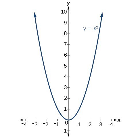
| \(x^2\) |  |
| \(\frac{x^3}{3} + C\) |  |
The graph of \(x^2\) shows a parabola, while the graph of its antiderivative \(\frac{x^3}{3} + C\) represents a cubic function.
Conclusion
The antiderivative of \(x^2\) is a fundamental concept in calculus, providing insights into the area under curves and the behavior of polynomial functions.
READ MORE:
Introduction to Antiderivatives
Antiderivatives, also known as indefinite integrals, are fundamental concepts in calculus. They represent the reverse process of differentiation. If a function \( F(x) \) is an antiderivative of \( f(x) \), then the derivative of \( F(x) \) is \( f(x) \). In other words, \( F'(x) = f(x) \). Antiderivatives are essential in solving various problems in physics, engineering, and other fields where integration is required to find areas, volumes, and other quantities.
The general form of an antiderivative of a function \( f(x) \) is given by \( F(x) + C \), where \( C \) is a constant. This constant arises because the differentiation of a constant is zero, meaning any constant added to an antiderivative will also be an antiderivative.
To understand the concept better, consider the power rule for integration: if \( f(x) = x^n \), where \( n \neq -1 \), then the antiderivative of \( f(x) \) is \( \frac{x^{n+1}}{n+1} + C \). For example, the antiderivative of \( x^2 \) is \( \frac{x^3}{3} + C \).
Antiderivatives are crucial for solving differential equations, which are equations involving derivatives. Many physical phenomena, such as motion under gravity or electrical circuits, can be described using differential equations. Finding antiderivatives allows us to solve these equations and understand the underlying behavior of the systems.
In summary, antiderivatives provide a way to 'reverse' differentiation and are indispensable in various mathematical applications. Understanding how to find and use antiderivatives opens up a wide range of possibilities in both theoretical and applied mathematics.
Understanding the Antiderivative of \(x^2\)
The antiderivative, or indefinite integral, of a function is a fundamental concept in calculus. It represents the inverse operation of differentiation, essentially "undoing" the process of finding a derivative. In this section, we will explore the antiderivative of \(x^2\) in detail.
To find the antiderivative of \(x^2\), we use the power rule for integration. The power rule states:
\[
\int x^n \, dx = \frac{x^{n+1}}{n+1} + C \quad \text{for} \, n \neq -1
\]
Applying this rule to \(x^2\):
- Identify the exponent \(n\) in \(x^2\). Here, \(n = 2\).
- Increase the exponent by 1: \(n + 1 = 2 + 1 = 3\).
- Divide \(x^{n+1}\) by the new exponent: \(\frac{x^3}{3}\).
- Don't forget to add the constant of integration \(C\), which accounts for any constant term that could have been differentiated to zero.
Thus, the antiderivative of \(x^2\) is:
\[
\int x^2 \, dx = \frac{x^3}{3} + C
\]
This result can be interpreted geometrically as the area under the curve \(y = x^2\) from a point to another point on the x-axis, plus an arbitrary constant. Understanding and computing antiderivatives is a critical skill in calculus, providing the foundation for solving many problems involving areas, volumes, and other quantities derived from functions.
Mathematical Definition and Rules
The antiderivative, also known as the indefinite integral, of a function is a fundamental concept in calculus. It represents the reverse process of differentiation. For a given function \(f(x)\), its antiderivative is a function \(F(x)\) such that \(F'(x) = f(x)\). The process of finding the antiderivative is known as antidifferentiation or integration.
Basic Rules of Antidifferentiation
- Constant Rule: The antiderivative of a constant \(c\) is \(cx + C\), where \(C\) is the constant of integration.
- Power Rule: The antiderivative of \(x^n\) is \(\frac{x^{n+1}}{n+1} + C\) for any real number \(n \neq -1\).
- Sum/Difference Rule: The antiderivative of a sum or difference of functions is the sum or difference of their antiderivatives.
Example: Antiderivative of \(x^2\)
- Identify the function: \(f(x) = x^2\).
- Apply the Power Rule: Using the rule \(\int x^n \, dx = \frac{x^{n+1}}{n+1} + C\), we set \(n = 2\).
- Compute the antiderivative: \(\int x^2 \, dx = \frac{x^{2+1}}{2+1} + C = \frac{x^3}{3} + C\).
Common Antiderivative Rules
| Function | Antiderivative |
|---|---|
| \(x^n\) | \(\frac{x^{n+1}}{n+1} + C\) for \(n \neq -1\) |
| \(e^x\) | \(e^x + C\) |
| \(\sin x\) | \(-\cos x + C\) |
| \(\cos x\) | \(\sin x + C\) |
| \(\frac{1}{x}\) | \(\ln |x| + C\) |
Understanding these rules and how to apply them is crucial for solving a variety of integration problems in calculus. Each function has specific rules that, when applied correctly, make finding antiderivatives straightforward.
Step-by-Step Solution for \(\int x^2 \, dx\)
The antiderivative of \(x^2\) involves finding the function whose derivative is \(x^2\). This process is known as integration. Follow these detailed steps to solve \(\int x^2 \, dx\):
- Identify the Power Rule: The power rule for integration states that \(\int x^n \, dx = \frac{x^{n+1}}{n+1} + C\) for any real number \(n \neq -1\).
- Apply the Power Rule: In this case, \(n = 2\). Substitute \(n\) into the power rule formula: \[ \int x^2 \, dx = \frac{x^{2+1}}{2+1} + C = \frac{x^3}{3} + C \]
- Simplify the Expression: The result simplifies to: \[ \frac{x^3}{3} + C \] Here, \(C\) represents the constant of integration, which accounts for any constant term that would disappear upon differentiation.
- Verification: To verify, differentiate \(\frac{x^3}{3} + C\) and ensure it equals \(x^2\): \[ \frac{d}{dx} \left( \frac{x^3}{3} + C \right) = x^2 \] The differentiation confirms that our antiderivative is correct.
Thus, the antiderivative of \(x^2\) is \(\frac{x^3}{3} + C\).
Examples and Applications
The antiderivative of \(x^2\), given by \(\int x^2 \, dx\), is a fundamental concept in calculus with various practical applications. Here, we explore some examples and applications of finding the antiderivative of \(x^2\).
Example 1: Basic Calculation
To find the antiderivative of \(x^2\), we use the power rule for integration:
\[
\int x^2 \, dx = \frac{x^{2+1}}{2+1} + C = \frac{x^3}{3} + C
\]
Here, \(C\) is the constant of integration.
Example 2: Area Under a Curve
Consider the function \(f(x) = x^2\). To find the area under the curve from \(x = a\) to \(x = b\), we calculate the definite integral:
\[
\int_a^b x^2 \, dx = \left[ \frac{x^3}{3} \right]_a^b = \frac{b^3}{3} - \frac{a^3}{3}
\]
This provides the exact area between the curve and the x-axis over the interval \([a, b]\).
Example 3: Physics Application - Kinematics
In kinematics, the position \(s(t)\) of an object moving with a constant acceleration \(a\) can be derived from the acceleration function. If the acceleration \(a(t) = 2\) (i.e., constant), the velocity \(v(t)\) is the antiderivative of \(a(t)\):
\[
v(t) = \int 2 \, dt = 2t + C_1
\]
Next, the position \(s(t)\) is the antiderivative of \(v(t)\):
\[
s(t) = \int (2t + C_1) \, dt = t^2 + C_1 t + C_2
\]
Here, \(C_1\) and \(C_2\) are constants determined by initial conditions.
Application in Economics
The concept of antiderivatives is also used in economics, for instance, in finding consumer and producer surplus. If \(D(x)\) represents the demand function and \(S(x)\) the supply function, the consumer surplus is the area between the demand curve and the price level. For example, if \(D(x) = 100 - x^2\), the consumer surplus when the price level is \(P = 20\) is:
\[
\text{Consumer Surplus} = \int_0^{x_P} (100 - x^2) \, dx - Px_P
\]
Where \(x_P\) is the quantity demanded at price \(P\).
Practice Problems
- Calculate \(\int x^2 \, dx\) and evaluate it from \(x = 1\) to \(x = 4\).
- Find the antiderivative of \(3x^2 - 4x + 5\).
- In a physics problem, if an object’s velocity is given by \(v(t) = 3t^2\), find the position function \(s(t)\) given that \(s(0) = 0\).
Conclusion
The antiderivative of \(x^2\) is a versatile tool in various fields such as physics, engineering, and economics. Understanding how to compute and apply it helps solve practical problems related to areas under curves, kinematic equations, and economic surplus calculations.
Common Mistakes to Avoid
When working with antiderivatives, particularly with functions like \(x^2\), it's important to be aware of common mistakes to avoid. Here are some typical errors and tips to help you steer clear of them:
- Forgetting the Constant of Integration:
One of the most common mistakes is forgetting to add the constant of integration \(C\). The antiderivative of \(x^2\) is \(\frac{x^3}{3} + C\), where \(C\) represents an arbitrary constant. This constant is crucial because it accounts for the fact that there are infinitely many antiderivatives for a given function, differing only by a constant.
- Incorrect Application of the Power Rule:
The power rule for integration states that \(\int x^n \, dx = \frac{x^{n+1}}{n+1} + C\). A common mistake is to incorrectly apply this rule. For example, some students might incorrectly integrate \(x^2\) as \(\frac{x^3}{2}\) instead of the correct \(\frac{x^3}{3}\).
- Misinterpreting the Variable:
Ensure that you correctly identify and integrate with respect to the variable given. If the problem states to integrate \(x^2\) with respect to \(x\), do not mistakenly integrate with respect to another variable.
- Sign Errors:
While integrating, especially when dealing with subtraction or more complex expressions, be cautious of sign errors. For example, correctly applying the power rule to \(-x^2\) would yield \(-\frac{x^3}{3} + C\), not \(\frac{-x^3}{3} + C\).
- Incorrect Handling of Constants:
When integrating a function with a constant multiplier, remember to apply the constant correctly. For example, the integral of \(5x^2\) is \(5 \cdot \frac{x^3}{3} + C\), which simplifies to \(\frac{5x^3}{3} + C\).
- Confusing Antiderivative with Definite Integral:
Remember that finding an antiderivative gives you a general form of the original function plus a constant, while a definite integral calculates the net area under a curve between specific bounds, resulting in a numerical value.
By keeping these common mistakes in mind and practicing regularly, you can improve your integration skills and avoid these pitfalls.
Advanced Techniques in Antidifferentiation
While basic techniques such as the power rule are essential for finding antiderivatives, advanced techniques are necessary for more complex functions. Here, we will explore several advanced methods used in antidifferentiation.
1. Integration by Parts
Integration by parts is a technique derived from the product rule of differentiation. It is used to integrate the product of two functions. The formula is given by:
\[
\int u \, dv = uv - \int v \, du
\]
where \(u\) and \(dv\) are differentiable functions of \(x\).
Steps to apply integration by parts:
- Choose \(u\) and \(dv\) from the integral \(\int u \, dv\).
- Differentiate \(u\) to find \(du\).
- Integrate \(dv\) to find \(v\).
- Substitute into the formula \(\int u \, dv = uv - \int v \, du\).
2. Trigonometric Substitution
This technique is useful for integrals involving square roots of quadratic expressions. The basic idea is to use trigonometric identities to simplify the integral. Common substitutions include:
- \(x = a \sin(\theta)\) for \(\sqrt{a^2 - x^2}\)
- \(x = a \tan(\theta)\) for \(\sqrt{a^2 + x^2}\)
- \(x = a \sec(\theta)\) for \(\sqrt{x^2 - a^2}\)
Steps to apply trigonometric substitution:
- Choose the appropriate trigonometric substitution based on the form of the integrand.
- Rewrite the integral in terms of the trigonometric function.
- Simplify and integrate using trigonometric identities.
- Convert back to the original variable using inverse trigonometric functions.
3. Partial Fraction Decomposition
Partial fraction decomposition is used to integrate rational functions (ratios of polynomials). The technique involves breaking down a complex rational function into simpler fractions that are easier to integrate. The steps are:
- Factor the denominator of the rational function.
- Express the integrand as a sum of partial fractions.
- Find the coefficients of the partial fractions by solving a system of equations.
- Integrate each partial fraction separately.
4. Improper Integrals
Improper integrals involve integrating functions over an infinite interval or integrands with infinite discontinuities. The technique involves taking limits to evaluate these integrals. For example:
\[
\int_{a}^{\infty} f(x) \, dx = \lim_{b \to \infty} \int_{a}^{b} f(x) \, dx
\]
Steps to evaluate improper integrals:
- Rewrite the improper integral as a limit of definite integrals.
- Evaluate the definite integral within the limit.
- Take the limit of the result.
5. Numerical Integration
When an antiderivative cannot be found analytically, numerical methods such as the Trapezoidal Rule, Simpson's Rule, and Riemann sums can be used to approximate the value of the integral. These methods involve approximating the area under the curve with simpler geometric shapes.
- Trapezoidal Rule: Approximates the area under the curve using trapezoids.
- Simpson's Rule: Uses parabolic segments to approximate the area under the curve.
- Riemann Sums: Approximates the area under the curve using rectangles.
Each method involves dividing the interval of integration into smaller subintervals and summing the areas of the shapes used in the approximation.
By mastering these advanced techniques, you can tackle a wide range of integrals that are not easily solvable using basic methods.
Applications in Physics and Engineering
The antiderivative of \(x^2\), which is \(\frac{1}{3}x^3 + C\), has numerous applications in both physics and engineering. These applications often involve calculating areas, volumes, and solving differential equations that describe physical phenomena. Here are some detailed applications:
-
1. Calculating Areas Under Curves
In physics, determining the area under a curve is essential for finding quantities such as work done by a force. For example, if the force applied varies with displacement \(x\) as \(F(x) = x^2\), the work done \(W\) from \(x = 0\) to \(x = a\) can be found by integrating the force function:
\[
W = \int_0^a x^2 \, dx = \left[ \frac{1}{3}x^3 \right]_0^a = \frac{1}{3}a^3
\] -
2. Centroid and Center of Mass Calculations
In engineering, the centroid of an area or the center of mass of a solid object is often required. For a parabolic lamina described by \(y = x^2\) between \(x = 0\) and \(x = b\), the centroid \((\bar{x}, \bar{y})\) can be found using the following integrals:
\[
\bar{x} = \frac{\int_0^b x \cdot x^2 \, dx}{\int_0^b x^2 \, dx} = \frac{\int_0^b x^3 \, dx}{\frac{1}{3}b^3} = \frac{\left[ \frac{1}{4}x^4 \right]_0^b}{\frac{1}{3}b^3} = \frac{\frac{1}{4}b^4}{\frac{1}{3}b^3} = \frac{3}{4}b
\]
\[
\bar{y} = \frac{1}{2} \cdot \frac{\int_0^b (x^2)^2 \, dx}{\int_0^b x^2 \, dx} = \frac{1}{2} \cdot \frac{\int_0^b x^4 \, dx}{\frac{1}{3}b^3} = \frac{1}{2} \cdot \frac{\left[ \frac{1}{5}x^5 \right]_0^b}{\frac{1}{3}b^3} = \frac{1}{2} \cdot \frac{\frac{1}{5}b^5}{\frac{1}{3}b^3} = \frac{3}{10}b
\] -
3. Volume of Solids of Revolution
In engineering, finding the volume of a solid of revolution is a common task. For a solid formed by rotating \(y = x^2\) about the x-axis from \(x = 0\) to \(x = a\), the volume \(V\) can be found using the disc method:
\[
V = \pi \int_0^a (x^2)^2 \, dx = \pi \int_0^a x^4 \, dx = \pi \left[ \frac{1}{5}x^5 \right]_0^a = \frac{\pi}{5}a^5
\] -
4. Solving Differential Equations
In physics, many problems involve solving differential equations. For example, consider a simple harmonic oscillator where the acceleration \(a\) is proportional to the displacement \(x\), and given by \(a = -kx\). The velocity \(v\) as a function of displacement can be found by integrating:
\[
v = \int a \, dx = -k \int x \, dx = -k \left( \frac{1}{2}x^2 + C \right)
\]For more complex systems, higher-order differential equations involving terms like \(x^2\) may appear, requiring integration to find solutions.
Practical Problems and Solutions
The antiderivative of \(x^2\) is a fundamental concept in calculus with numerous practical applications. Here are some example problems and their solutions to help you understand how to apply the antiderivative of \(x^2\) in various scenarios.
Example 1: Basic Antiderivative Calculation
Find the antiderivative of \(f(x) = x^2\).
Solution:
Using the power rule for integration, we have:
\[
\int x^2 \, dx = \frac{1}{3}x^3 + C
\]
where \(C\) is the constant of integration.
Example 2: Initial Value Problem
Solve the initial value problem: \(\frac{dy}{dx} = x^2\), with \(y(1) = 3\).
Solution:
- First, find the general antiderivative: \[ y = \int x^2 \, dx = \frac{1}{3}x^3 + C \]
- Use the initial condition \(y(1) = 3\) to find \(C\): \[ 3 = \frac{1}{3}(1)^3 + C \implies C = 3 - \frac{1}{3} = \frac{8}{3} \]
- Thus, the particular solution is: \[ y = \frac{1}{3}x^3 + \frac{8}{3} \]
Example 3: Area Under a Curve
Find the area under the curve \(f(x) = x^2\) from \(x = 0\) to \(x = 2\).
Solution:
- Set up the definite integral: \[ \int_{0}^{2} x^2 \, dx \]
- Evaluate the antiderivative at the bounds: \[ \left[ \frac{1}{3}x^3 \right]_{0}^{2} = \frac{1}{3}(2)^3 - \frac{1}{3}(0)^3 = \frac{8}{3} - 0 = \frac{8}{3} \]
- The area under the curve is \(\frac{8}{3}\) square units.
Example 4: Physics Application - Kinematics
A particle moves along a line so that its acceleration \(a(t)\) is given by \(a(t) = t^2\). Find the velocity \(v(t)\) if the initial velocity \(v(0) = 4\) m/s.
Solution:
- Integrate the acceleration to find the velocity: \[ v(t) = \int t^2 \, dt = \frac{1}{3}t^3 + C \]
- Use the initial condition \(v(0) = 4\) to find \(C\): \[ 4 = \frac{1}{3}(0)^3 + C \implies C = 4 \]
- Thus, the velocity function is: \[ v(t) = \frac{1}{3}t^3 + 4 \]
Example 5: Engineering Application - Beam Deflection
In structural engineering, the deflection \(y(x)\) of a beam under a uniformly distributed load can be modeled by the equation \(y''(x) = \frac{w}{EI} x^2\), where \(w\) is the load per unit length, \(E\) is the modulus of elasticity, and \(I\) is the moment of inertia. Find the deflection if \(y(0) = 0\) and \(y'(0) = 0\).
Solution:
- Integrate twice to find the deflection \(y(x)\): \[ y'(x) = \int \frac{w}{EI} x^2 \, dx = \frac{w}{EI} \cdot \frac{1}{3}x^3 + C_1 \] \[ y(x) = \int \left( \frac{w}{EI} \cdot \frac{1}{3}x^3 + C_1 \right) \, dx = \frac{w}{EI} \cdot \frac{1}{12}x^4 + C_1 x + C_2 \]
- Use the boundary conditions to solve for \(C_1\) and \(C_2\): \[ y'(0) = 0 \implies C_1 = 0 \] \[ y(0) = 0 \implies C_2 = 0 \]
- Thus, the deflection function is: \[ y(x) = \frac{w}{EI} \cdot \frac{1}{12}x^4 \]
These examples illustrate how the antiderivative of \(x^2\) can be used to solve practical problems in mathematics, physics, and engineering.
Frequently Asked Questions (FAQs)
-
What is the antiderivative of \(x^2\)?
The antiderivative of \(x^2\) is \(\frac{1}{3}x^3 + C\), where \(C\) is the constant of integration. This is derived using the power rule for integration, which states that \(\int x^n \, dx = \frac{x^{n+1}}{n+1} + C\).
-
Why is there a constant \(C\) in the antiderivative?
The constant \(C\) represents the family of all possible antiderivatives. Since the derivative of a constant is zero, any constant added to the antiderivative function will also have the same derivative.
-
How do you verify the antiderivative of \(x^2\)?
You can verify the antiderivative by differentiating it. For example, differentiate \(\frac{1}{3}x^3 + C\):
\[
\frac{d}{dx} \left(\frac{1}{3}x^3 + C\right) = x^2
\]
The result is the original function, confirming the antiderivative is correct. -
What is the significance of finding antiderivatives?
Antiderivatives are essential in solving problems related to area under curves, displacement from velocity, and other applications in physics and engineering where the integral of a function is needed to find cumulative quantities.
-
Can the antiderivative be used to solve practical problems?
Yes, antiderivatives are used to solve various practical problems, such as calculating the area under a curve, determining the displacement from velocity in physics, and finding the total accumulated quantity over an interval.
-
How do you apply the power rule for integration?
The power rule for integration states that \(\int x^n \, dx = \frac{x^{n+1}}{n+1} + C\), where \(n \neq -1\). For example, to integrate \(x^2\):
\[
\int x^2 \, dx = \frac{x^{2+1}}{2+1} + C = \frac{x^3}{3} + C
\] -
What are some common mistakes to avoid when finding antiderivatives?
Common mistakes include forgetting to add the constant of integration \(C\), applying the power rule incorrectly, and not simplifying the integrand properly before integrating.
Additional Resources for Further Learning
To deepen your understanding of antiderivatives and their applications, here are some valuable resources that cover a range of topics, from basic principles to advanced techniques:
- Khan Academy: An extensive collection of video tutorials and practice exercises on antiderivatives and integration. This platform is great for visual learners and offers step-by-step solutions. Visit the .
- Paul's Online Math Notes: A comprehensive set of notes and examples on calculus topics, including antiderivatives. This resource is ideal for students looking for detailed explanations and example problems. Explore more at .
- Wolfram Alpha: An interactive computational tool that allows you to input integrals and see step-by-step solutions. It's useful for checking your work and understanding the integration process. Try it out at .
- MIT OpenCourseWare: Free lecture notes, exams, and videos from MIT’s calculus courses. These materials cover a broad range of topics and are suitable for both self-study and supplementary learning. Access the materials at .
- Math Is Fun: A user-friendly website that provides explanations and examples of calculus concepts in an easy-to-understand manner. It's perfect for beginners who need a straightforward introduction to antiderivatives. Visit .
- Coursera and edX: Online learning platforms offering courses from top universities on calculus and related subjects. These courses often include video lectures, assignments, and discussion forums. Check out calculus courses on and .
- Mathematics LibreTexts: A collaborative platform providing high-quality, open-access textbooks on mathematics. The site includes a dedicated section on antiderivatives and integration techniques. Visit .
These resources should help you gain a better grasp of antiderivatives, practice solving integrals, and explore their various applications. Happy learning!
READ MORE:
Video hướng dẫn chi tiết cách tính tích phân của x bình phương, giúp bạn hiểu rõ và áp dụng vào các bài toán thực tế.
Cách tính tích phân của x bình phương