Topic what is the null hypothesis for a chi-square test: The null hypothesis for a Chi-Square test is crucial in determining whether observed data significantly deviates from expected outcomes. This article provides a clear explanation of the null hypothesis, its role in Chi-Square tests, and how it helps in analyzing relationships between categorical variables. Learn how to apply this statistical tool effectively in your data analysis.
Table of Content
- Understanding the Null Hypothesis for a Chi-Square Test
- Introduction to the Chi-Square Test
- Understanding the Null Hypothesis
- Types of Chi-Square Tests
- Formulating the Null Hypothesis
- Mathematical Representation of the Null Hypothesis
- Calculating the Chi-Square Statistic
- Interpreting Results
- Common Applications
- Chi-Square Test of Independence
- Chi-Square Goodness of Fit Test
- Assumptions and Limitations
- Example Scenarios
- YOUTUBE: Tìm hiểu về kiểm tra Chi-Square và giả thuyết không để phân biệt giữa các biến trong dữ liệu danh mục.
Understanding the Null Hypothesis for a Chi-Square Test
The Chi-Square test is a statistical method used to determine if there is a significant association between categorical variables. The null hypothesis is a critical part of this test. Here, we explore what the null hypothesis is and how it is formulated in a Chi-Square test.
Definition of the Null Hypothesis
The null hypothesis (\(H_0\)) for a Chi-Square test states that there is no significant difference between the observed and expected frequencies in one or more categories. In other words, any observed differences are due to random chance.
- Chi-Square Test of Independence: \(H_0\): The variables are independent.
- Chi-Square Goodness of Fit Test: \(H_0\): The observed frequencies match the expected frequencies.
Mathematical Representation
The null hypothesis can be represented mathematically as:
$$H_0: O_i = E_i$$
where \(O_i\) are the observed frequencies and \(E_i\) are the expected frequencies. The Chi-Square statistic is calculated as:
$$\chi^2 = \sum \frac{(O_i - E_i)^2}{E_i}$$
This statistic follows a Chi-Square distribution with degrees of freedom equal to the number of categories minus one.
Interpreting the Null Hypothesis
When performing a Chi-Square test, the null hypothesis is either rejected or not rejected based on the p-value:
- If the p-value is less than the significance level (e.g., 0.05), we reject \(H_0\), indicating a significant association between the variables.
- If the p-value is greater than the significance level, we fail to reject \(H_0\), suggesting no significant association between the variables.
Conclusion
In summary, the null hypothesis in a Chi-Square test provides a baseline assumption that there is no relationship between the categorical variables being tested. Rejecting or failing to reject this hypothesis helps in understanding the relationship between these variables in the given data.
| Test Type | Null Hypothesis (\(H_0\)) |
|---|---|
| Chi-Square Test of Independence | The variables are independent. |
| Chi-Square Goodness of Fit Test | The observed frequencies match the expected frequencies. |
READ MORE:
Introduction to the Chi-Square Test
The Chi-Square test is a statistical method used to determine if there is a significant association between categorical variables or if a sample matches an expected distribution. This test is commonly used in hypothesis testing to analyze data in the form of frequency counts.
The Chi-Square test has two main types:
- Chi-Square Test of Independence: This test assesses whether two categorical variables are independent of each other. It is used to determine if there is a significant association between the variables in a contingency table.
- Chi-Square Goodness of Fit Test: This test evaluates how well an observed distribution matches an expected distribution. It is used to determine if the frequencies of different categories fit a specific theoretical distribution.
Key steps in performing a Chi-Square test include:
- Formulate Hypotheses: Define the null hypothesis (\(H_0\)) and the alternative hypothesis (\(H_a\)).
- Collect Data: Gather the observed frequency counts for each category.
- Calculate Expected Frequencies: Determine the expected frequencies based on the null hypothesis.
- Compute Chi-Square Statistic: Use the formula: $$\chi^2 = \sum \frac{(O_i - E_i)^2}{E_i}$$ where \(O_i\) is the observed frequency and \(E_i\) is the expected frequency.
- Compare to Critical Value: Compare the calculated Chi-Square statistic to the critical value from the Chi-Square distribution table with the appropriate degrees of freedom.
- Make Decision: If the Chi-Square statistic is greater than the critical value, reject the null hypothesis. Otherwise, fail to reject the null hypothesis.
The Chi-Square test is widely used in various fields such as social sciences, marketing, and biology to analyze categorical data and draw meaningful conclusions about the relationships between variables or the fit of data to expected distributions.
Understanding the Null Hypothesis
The null hypothesis (\(H_0\)) in a Chi-Square test is a statement that assumes no effect or no association between the variables being tested. It serves as a starting point for statistical analysis and provides a baseline against which the observed data is compared. In Chi-Square tests, the null hypothesis helps determine whether any observed deviations from the expected frequencies are due to random chance or indicate a significant difference.
The formulation of the null hypothesis depends on the type of Chi-Square test being used:
- Chi-Square Test of Independence:
- Null Hypothesis (\(H_0\)): The variables are independent, meaning there is no association between them.
- Alternative Hypothesis (\(H_a\)): The variables are not independent, indicating a significant association between them.
- Chi-Square Goodness of Fit Test:
- Null Hypothesis (\(H_0\)): The observed frequencies match the expected frequencies, suggesting the data fits the specified distribution.
- Alternative Hypothesis (\(H_a\)): The observed frequencies do not match the expected frequencies, indicating the data does not fit the specified distribution.
To test the null hypothesis, follow these steps:
- Set Up Hypotheses: Clearly define the null and alternative hypotheses.
- Calculate Expected Frequencies: Determine the expected frequencies for each category based on the null hypothesis.
- Compute the Chi-Square Statistic: Use the formula: $$\chi^2 = \sum \frac{(O_i - E_i)^2}{E_i}$$ where \(O_i\) represents the observed frequencies, and \(E_i\) represents the expected frequencies.
- Determine Degrees of Freedom: Calculate the degrees of freedom (\(df\)), which typically equals the number of categories minus one for the goodness of fit test, or \((r-1) \times (c-1)\) for the test of independence, where \(r\) is the number of rows and \(c\) is the number of columns.
- Compare to Critical Value: Compare the calculated Chi-Square statistic to the critical value from the Chi-Square distribution table with the corresponding degrees of freedom.
- Draw Conclusion: If the Chi-Square statistic exceeds the critical value, reject the null hypothesis. Otherwise, fail to reject the null hypothesis.
In conclusion, the null hypothesis in a Chi-Square test plays a vital role in determining whether the observed data significantly deviates from what is expected under the assumption of no effect or no association. This process aids in making informed decisions based on statistical evidence.
Types of Chi-Square Tests
There are two main types of Chi-Square tests used in statistical analysis:
- Chi-Square Test of Independence: This test determines whether there is a significant association between two categorical variables. It is commonly used in contingency tables to evaluate if the observed frequency distribution differs from the expected distribution.
- Chi-Square Goodness of Fit Test: This test assesses whether the observed frequency distribution of a single categorical variable matches an expected distribution. It is useful for determining if a sample data set comes from a population with a specific distribution.
Chi-Square Test of Independence
The Chi-Square Test of Independence is used to examine the relationship between two categorical variables. The null hypothesis in this test states that the variables are independent, meaning there is no association between them.
- Formulate the null and alternative hypotheses:
- Null Hypothesis (\(H_0\)): The variables are independent.
- Alternative Hypothesis (\(H_a\)): The variables are not independent.
- Construct a contingency table to summarize the frequencies of different combinations of the variables.
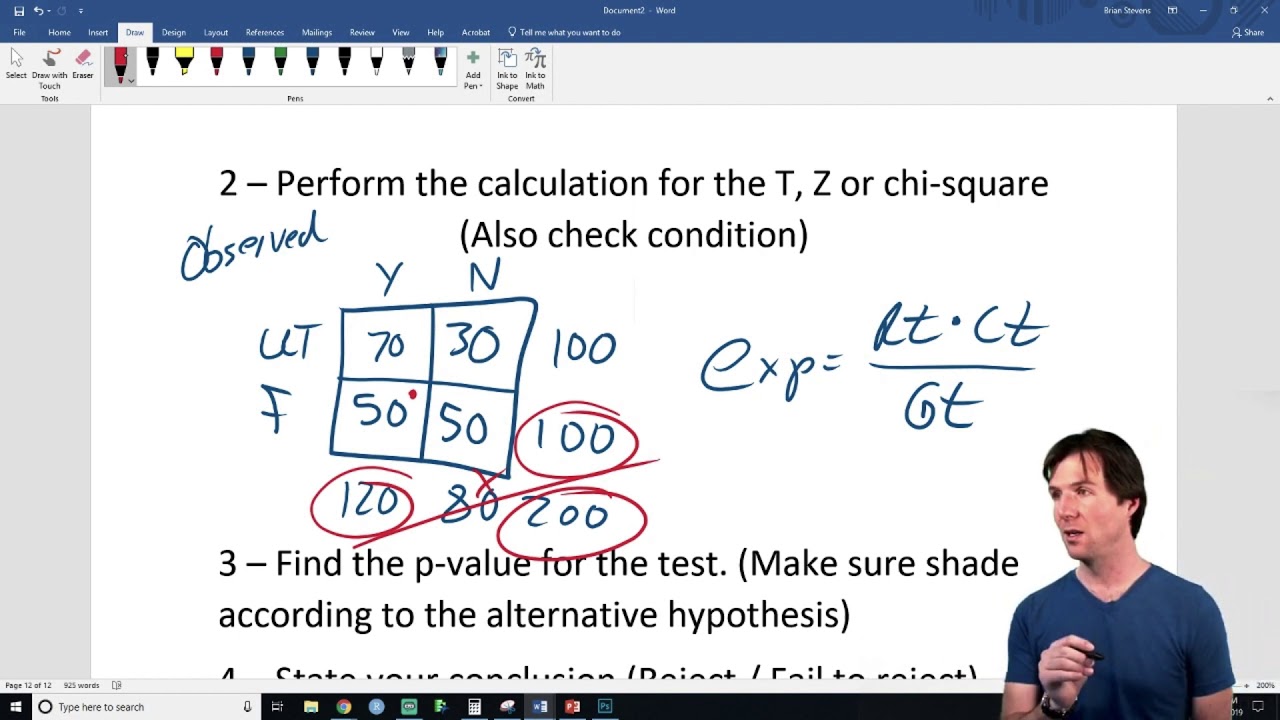
- Calculate the expected frequencies for each cell in the contingency table using the formula: \[ E_{ij} = \frac{(row\;total_i \times column\;total_j)}{grand\;total} \]
- Compute the Chi-Square statistic using the formula: \[ \chi^2 = \sum \frac{(O_{ij} - E_{ij})^2}{E_{ij}} \] where \(O_{ij}\) is the observed frequency and \(E_{ij}\) is the expected frequency.
- Compare the computed Chi-Square statistic to the critical value from the Chi-Square distribution table with appropriate degrees of freedom to determine the p-value.
- Draw a conclusion:
- If the p-value is less than the significance level (e.g., 0.05), reject the null hypothesis.
- If the p-value is greater than the significance level, do not reject the null hypothesis.
Chi-Square Goodness of Fit Test
The Chi-Square Goodness of Fit Test is used to determine if a sample data set fits a population with a specific distribution. The null hypothesis in this test states that the observed frequencies match the expected frequencies.
- Formulate the null and alternative hypotheses:
- Null Hypothesis (\(H_0\)): The observed frequencies fit the expected distribution.
- Alternative Hypothesis (\(H_a\)): The observed frequencies do not fit the expected distribution.
- Calculate the expected frequencies for each category based on the hypothesized distribution.
- Compute the Chi-Square statistic using the formula: \[ \chi^2 = \sum \frac{(O_i - E_i)^2}{E_i} \] where \(O_i\) is the observed frequency and \(E_i\) is the expected frequency.
- Compare the computed Chi-Square statistic to the critical value from the Chi-Square distribution table with the appropriate degrees of freedom to determine the p-value.
- Draw a conclusion:
- If the p-value is less than the significance level (e.g., 0.05), reject the null hypothesis.
- If the p-value is greater than the significance level, do not reject the null hypothesis.
Formulating the Null Hypothesis
In the context of Chi-Square tests, the null hypothesis is a critical component that represents a statement of no effect or no relationship between the variables being tested. Formulating the null hypothesis involves the following steps:
- Identify the Variables:
Determine the categorical variables involved in your study. For example, if you are studying the relationship between gender and voting preference, the variables would be 'gender' and 'voting preference'.
- State the Null Hypothesis (H0):
The null hypothesis typically states that there is no association between the variables or that the observed frequencies of occurrences are consistent with expected frequencies. For the Chi-Square Test of Independence, the null hypothesis can be stated as:
H0: There is no significant association between the two categorical variables.
For the Chi-Square Goodness of Fit Test, the null hypothesis can be stated as:
H0: The observed frequencies in each category are equal to the expected frequencies.
- Define the Alternative Hypothesis (Ha):
The alternative hypothesis states that there is an association between the variables or that the observed frequencies are different from the expected frequencies. For the Chi-Square Test of Independence, the alternative hypothesis can be stated as:
Ha: There is a significant association between the two categorical variables.
For the Chi-Square Goodness of Fit Test, the alternative hypothesis can be stated as:
Ha: The observed frequencies in each category are not equal to the expected frequencies.
Formulating the null hypothesis clearly and precisely is essential as it guides the direction of the statistical test and helps in interpreting the results accurately.
The steps involved in Chi-Square tests are as follows:
- Calculate the expected frequencies for each category based on the null hypothesis.
- Compute the Chi-Square statistic using the formula:
\[ \chi^2 = \sum \frac{(O_i - E_i)^2}{E_i} \] where \(O_i\) represents the observed frequency and \(E_i\) represents the expected frequency.
- Compare the calculated Chi-Square statistic to the critical value from the Chi-Square distribution table based on the degrees of freedom.
- Determine the p-value to assess the significance of the results. If the p-value is less than the chosen significance level (typically 0.05), reject the null hypothesis.
By following these steps, researchers can effectively test their hypotheses and draw meaningful conclusions from their data.
Mathematical Representation of the Null Hypothesis
The null hypothesis in a chi-square test is a statement that there is no significant difference between the observed and expected frequencies. Mathematically, this can be represented using the chi-square formula:
The chi-square test statistic is calculated as:
\[ \chi^2 = \sum \frac{(O_i - E_i)^2}{E_i} \]
- \(\chi^2\) is the chi-square test statistic.
- \(O_i\) represents the observed frequency for the \(i\)-th category.
- \(E_i\) represents the expected frequency for the \(i\)-th category, calculated under the null hypothesis.
The expected frequency (\(E_i\)) for each category is calculated as:
\[ E_i = \frac{\text{Row total} \times \text{Column total}}{\text{Grand total}} \]
Where:
- Row total is the total frequency of the row that the cell belongs to.
- Column total is the total frequency of the column that the cell belongs to.
- Grand total is the sum of all frequencies in the table.
Once the chi-square statistic (\(\chi^2\)) is computed, it is compared to the critical value from the chi-square distribution table with the appropriate degrees of freedom. The degrees of freedom (df) are calculated as:
\[ \text{df} = (r - 1) \times (c - 1) \]
- \(r\) is the number of rows.
- \(c\) is the number of columns.
If the chi-square statistic is greater than the critical value, the null hypothesis is rejected, indicating a significant difference between the observed and expected frequencies.
Calculating the Chi-Square Statistic
The chi-square statistic is used to determine whether there is a significant difference between the expected frequencies and the observed frequencies in one or more categories. Here are the detailed steps to calculate the chi-square statistic:
-
Define the null and alternative hypotheses:
- Null hypothesis (H0): Assumes that there is no significant difference between the expected and observed frequencies.
- Alternative hypothesis (HA): Assumes that there is a significant difference between the expected and observed frequencies.
-
Collect and organize the data:
Gather the observed frequencies (O) and determine the expected frequencies (E) based on the null hypothesis. Organize the data into a table:
Category Observed Frequency (O) Expected Frequency (E) (O - E) (O - E)2 (O - E)2 / E -
Calculate the chi-square statistic (X2):
The formula for the chi-square statistic is given by:
\[
X^2 = \sum \frac{(O_i - E_i)^2}{E_i}
\]Where:
- \(O_i\) = observed frequency for category \(i\)
- \(E_i\) = expected frequency for category \(i\)
- \(\sum\) = summation over all categories
Compute this value for each category and sum them up to get the chi-square statistic.
-
Determine the degrees of freedom (df):
Degrees of freedom for the chi-square test is calculated as:
\[
df = (number \, of \, categories - 1)
\] -
Compare the chi-square statistic to the critical value:
Using a chi-square distribution table, find the critical value based on the degrees of freedom and the chosen significance level (usually 0.05).
If the chi-square statistic exceeds the critical value, reject the null hypothesis. Otherwise, fail to reject the null hypothesis.
Here's an example calculation:
- Suppose we have observed frequencies: 15, 12, 9, 8, 8, 6 for six categories.
- Assume the expected frequency for each category is 10.
- Calculate the chi-square statistic:
- Category 1: \( (15 - 10)^2 / 10 = 2.5 \)
- Category 2: \( (12 - 10)^2 / 10 = 0.4 \)
- Category 3: \( (9 - 10)^2 / 10 = 0.1 \)
- Category 4: \( (8 - 10)^2 / 10 = 0.4 \)
- Category 5: \( (8 - 10)^2 / 10 = 0.4 \)
- Category 6: \( (6 - 10)^2 / 10 = 1.6 \)
- Sum these values: \(2.5 + 0.4 + 0.1 + 0.4 + 0.4 + 1.6 = 5.4\)
- Determine degrees of freedom: \(df = 6 - 1 = 5\)
- Compare to critical value from chi-square table. If 5.4 is less than the critical value (e.g., 11.07 for df=5, \(\alpha = 0.05\)), we fail to reject the null hypothesis.
This process allows researchers to statistically determine whether there is a significant difference between the observed data and what was expected.
Interpreting Results
Interpreting the results of a Chi-Square test involves several key steps to determine if the observed data significantly deviates from the expected data under the null hypothesis. Here is a detailed guide to interpreting Chi-Square test results:
-
Determine the Degrees of Freedom:
The degrees of freedom (df) for a Chi-Square test are calculated based on the number of categories in the data. For a Chi-Square test of independence, the formula is:
\[
\text{df} = (r - 1) \times (c - 1)
\]where \(r\) is the number of rows and \(c\) is the number of columns.
-
Calculate the P-Value:
The P-value indicates the probability that the observed differences are due to random chance. To find the P-value, compare your test statistic to the Chi-Square distribution table at the calculated degrees of freedom.
-
Compare P-Value to Significance Level:
Choose a significance level (commonly 0.05). If the P-value is less than or equal to the significance level, reject the null hypothesis. This means there is a statistically significant association between the variables.
-
Evaluate Observed vs. Expected Counts:
Examine the observed and expected counts in your data. Large discrepancies between these counts indicate a higher Chi-Square statistic and a greater likelihood of rejecting the null hypothesis.
-
Interpret the Results:
Based on the P-value and the observed vs. expected counts, draw conclusions about your hypothesis. For example:
- If \(P \leq \alpha\): Reject the null hypothesis and conclude that there is a significant association between the variables.
- If \(P > \alpha\): Fail to reject the null hypothesis and conclude that there is no significant association.
Here is a step-by-step example:
-
Observed and Expected Counts:
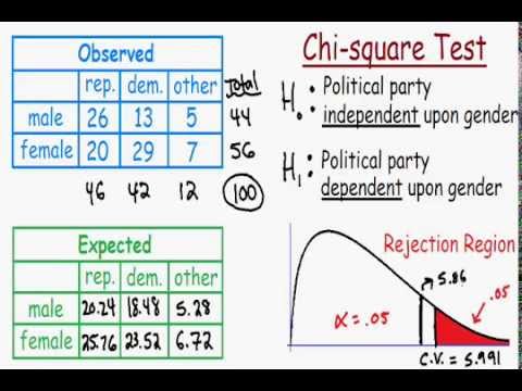
Imagine a study examining the relationship between two categorical variables: smoking status (smoker, non-smoker) and the presence of respiratory disease (yes, no).
Smoker Non-Smoker Disease Present 20 (15) 10 (15) Disease Absent 10 (15) 20 (15) Numbers in parentheses are expected counts.
-
Calculate Chi-Square Statistic:
The Chi-Square statistic is calculated as:
\[
\chi^2 = \sum \frac{(O - E)^2}{E}
\]For this example, it might yield a Chi-Square statistic of 6.67.
-
Degrees of Freedom:
With 2 rows and 2 columns, the degrees of freedom are:
\[
\text{df} = (2 - 1) \times (2 - 1) = 1
\] -
P-Value and Conclusion:
Using a Chi-Square distribution table, the P-value for 6.67 with 1 degree of freedom might be 0.01. Since 0.01 < 0.05, reject the null hypothesis, indicating a significant association between smoking status and respiratory disease.
Thus, interpreting Chi-Square results involves examining the P-value in context with your significance level and the observed and expected counts to draw meaningful conclusions about your data.
Common Applications
The Chi-Square test is widely used in various fields to analyze categorical data and test hypotheses about the relationships between categorical variables. Here are some common applications:
-
Social Sciences:
Researchers in sociology, psychology, political science, and other social sciences use the Chi-Square test to examine relationships between categorical variables. For example, it can be used to analyze survey responses, voting patterns, or the association between demographic variables and specific behaviors.
-
Market Research:
Market researchers use the Chi-Square test to analyze consumer preferences, brand loyalty, purchasing behavior, and market segmentation. It helps in understanding if there is a significant difference in consumer behavior across different groups.
-
Biology and Genetics:
In genetics, the Chi-Square test is used to study inheritance patterns, genetic linkage, allele frequencies, and the association between genetic traits and diseases.
-
Public Health:
Public health professionals use the Chi-Square test to analyze data related to disease prevalence, risk factors, and health outcomes. It helps assess associations between exposure variables and health outcomes in population studies.
-
Quality Control:
Quality control specialists use the Chi-Square test to analyze data from defect classification, product inspection, and quality assurance processes. It helps identify patterns and assess the effectiveness of process improvements.
-
Education Research:
Education researchers use the Chi-Square test to examine relationships between variables such as student performance and teaching methods. It can also be used to analyze survey data related to educational practices and outcomes.
The versatility and wide applicability of the Chi-Square test make it a valuable tool in statistical analysis for various domains, providing insights into relationships and differences between categorical variables.
Chi-Square Test of Independence
The Chi-Square Test of Independence is used to determine if there is a significant association between two categorical variables. This test assesses whether the distribution of sample categorical data matches an expected distribution under the null hypothesis.
Steps to Perform the Chi-Square Test of Independence
-
State the Hypotheses
- Null Hypothesis (\(H_0\)): There is no association between the two categorical variables. They are independent.
- Alternative Hypothesis (\(H_a\)): There is an association between the two categorical variables. They are not independent.
-
Formulate an Analysis Plan
- Determine the significance level (\(\alpha\)), commonly set at 0.05.
- Select the appropriate test method, which is the Chi-Square Test of Independence.
-
Analyze Sample Data
- Construct a contingency table from the sample data.
- Calculate the expected frequencies for each cell in the table using: \[ E_{ij} = \frac{(row\ total\ for\ row\ i) \times (column\ total\ for\ column\ j)}{grand\ total} \]
- Compute the Chi-Square statistic: \[ \chi^2 = \sum \frac{(O_{ij} - E_{ij})^2}{E_{ij}} \] where \(O_{ij}\) is the observed frequency and \(E_{ij}\) is the expected frequency.
-
Interpret Results
- Determine the degrees of freedom: \[ df = (r-1) \times (c-1) \] where \(r\) is the number of rows and \(c\) is the number of columns.
- Find the critical value from the Chi-Square distribution table based on the degrees of freedom and significance level.
- Compare the Chi-Square statistic to the critical value:
- If \(\chi^2\) is greater than the critical value, reject the null hypothesis.
- If \(\chi^2\) is less than or equal to the critical value, do not reject the null hypothesis.
By following these steps, you can determine whether there is a significant association between the two categorical variables in your data, thus concluding whether they are independent or not.
Chi-Square Goodness of Fit Test
The Chi-Square Goodness of Fit Test is used to determine whether a sample data matches a population with a specific distribution. This test is particularly useful when dealing with categorical data.
To conduct a Chi-Square Goodness of Fit Test, follow these steps:
-
State the Hypotheses
- Null Hypothesis (\(H_0\)): The sample data fits the specified distribution.
- Alternative Hypothesis (\(H_a\)): The sample data does not fit the specified distribution.
-
Determine the Expected Frequencies
Calculate the expected frequency for each category using the formula:
\[ E_i = N \times p_i \]
where \(E_i\) is the expected frequency for category \(i\), \(N\) is the total number of observations, and \(p_i\) is the probability of category \(i\) according to the null hypothesis.
-
Calculate the Chi-Square Statistic
The Chi-Square statistic is calculated using the formula:
\[ \chi^2 = \sum \frac{(O_i - E_i)^2}{E_i} \]
where \(O_i\) is the observed frequency for category \(i\), and \(E_i\) is the expected frequency for category \(i\).
-
Determine the Degrees of Freedom
The degrees of freedom for this test is calculated as:
\[ df = k - 1 \]
where \(k\) is the number of categories.
-
Compare the Chi-Square Statistic to the Critical Value
Find the critical value from the Chi-Square distribution table using the calculated degrees of freedom and the chosen significance level (\(\alpha\)). If the Chi-Square statistic is greater than the critical value, reject the null hypothesis.
Example: Suppose a company claims that 30% of its products are of type A, 50% are of type B, and 20% are of type C. To test this claim, a sample of 100 products is taken, and the observed frequencies are 32, 47, and 21 for types A, B, and C, respectively.
1. State the hypotheses:
- \(H_0\): The distribution of products is 30% type A, 50% type B, and 20% type C.
- \(H_a\): The distribution of products is not as claimed.
2. Calculate the expected frequencies:
- \(E_A = 100 \times 0.30 = 30\)
- \(E_B = 100 \times 0.50 = 50\)
- \(E_C = 100 \times 0.20 = 20\)
3. Calculate the Chi-Square statistic:
\[ \chi^2 = \frac{(32-30)^2}{30} + \frac{(47-50)^2}{50} + \frac{(21-20)^2}{20} = 0.1333 + 0.18 + 0.05 = 0.3633 \]
4. Determine the degrees of freedom:
\[ df = 3 - 1 = 2 \]
5. Compare the Chi-Square statistic to the critical value:
For \(\alpha = 0.05\) and \(df = 2\), the critical value from the Chi-Square distribution table is 5.991. Since 0.3633 < 5.991, we fail to reject \(H_0\).
Conclusion: There is not enough evidence to reject the null hypothesis. The sample data fits the specified distribution.
Assumptions and Limitations
The Chi-Square Test relies on several key assumptions to produce valid results. Understanding and meeting these assumptions is critical for accurate and reliable outcomes.
Assumptions
- Independence of Observations: The observations must be independent of each other. This means that the occurrence of one event does not affect the probability of another.
- Random Sampling: The data should be collected through a random sampling method to ensure each member of the population has an equal chance of being selected.
- Categorical Data: The data should be in the form of frequencies or counts of categories, not percentages or continuous data.
- Expected Frequency: Each cell in the contingency table should have an expected frequency of at least 5. If more than 20% of the cells have expected frequencies less than 5, the test may not be valid.
- Mutually Exclusive Categories: Each observation should fall into only one category, ensuring that the categories are mutually exclusive.
Limitations
- Data Type: The Chi-Square Test is suitable only for categorical data. Continuous data must be appropriately categorized before applying the test.
- Sample Size: The test requires a sufficiently large sample size to produce accurate results. Small sample sizes can lead to unreliable outcomes.
- Sensitivity to Sparse Data: The test can give misleading results if some cells have very low frequencies or are empty. In such cases, other tests like Fisher's exact test might be preferred.
- No Measure of Strength: While the test can indicate whether an association exists, it does not measure the strength or direction of the association. Additional measures like Cramer's V or Phi are needed for this purpose.
- Handling of Missing Data: The Chi-Square Test is not robust against missing data. Missing values must be appropriately handled before performing the test.
By adhering to these assumptions and understanding its limitations, we can ensure that the Chi-Square Test is used correctly and its results are valid. Misunderstanding or violating these assumptions can lead to inaccurate conclusions.
Example Scenarios
To illustrate the application of the chi-square test, let's consider two example scenarios: one for the Chi-Square Test of Independence and another for the Chi-Square Goodness of Fit Test.
Chi-Square Test of Independence
Suppose a researcher wants to determine if there is an association between education level and marital status among adults in a city. The researcher collects data and organizes it into a contingency table as follows:
| Education Level | Never Married | Married | Divorced | Total |
|---|---|---|---|---|
| High School | 30 | 50 | 20 | 100 |
| College | 40 | 60 | 30 | 130 |
| Graduate | 20 | 30 | 10 | 60 |
| Total | 90 | 140 | 60 | 290 |
The null hypothesis (\(H_0\)) is that education level and marital status are independent. Using the chi-square test, we calculate the expected frequencies and compare them to the observed frequencies to determine if there is a significant association between the two variables.
Chi-Square Goodness of Fit Test
In another scenario, an analyst wants to determine if the distribution of car accidents at a busy intersection follows a Poisson distribution. The analyst records the number of accidents per month over 50 months, and the observed counts are as follows:
| Number of Accidents | Observed Frequency |
|---|---|
| 0 | 12 |
| 1 | 15 |
| 2 | 10 |
| 3 | 8 |
| 4 | 3 |
| 5 | 2 |
The null hypothesis (\(H_0\)) is that the data follow a Poisson distribution. The expected frequencies are calculated based on the Poisson distribution, and the chi-square statistic is used to compare the observed and expected frequencies. If the p-value is greater than the significance level, we fail to reject the null hypothesis, suggesting that the data follow the Poisson distribution.

Tìm hiểu về kiểm tra Chi-Square và giả thuyết không để phân biệt giữa các biến trong dữ liệu danh mục.
Kiểm Tra Chi-Square
READ MORE:
Tìm hiểu về thống kê Chi-Square và cách sử dụng để kiểm tra giả thuyết trong môn Thống Kê AP từ Khan Academy.
Thống Kê Chi-Square cho Kiểm Tra Giả Thuyết | AP Statistics | Khan Academy
:max_bytes(150000):strip_icc()/Chi-SquareStatistic_Final_4199464-7eebcd71a4bf4d9ca1a88d278845e674.jpg)