Topic null hypothesis for chi square test: The null hypothesis in the chi-square test is a fundamental concept in statistics, used to determine if there is a significant association between categorical variables. This introduction will explore its importance, application, and interpretation in statistical analysis, helping you make informed decisions based on data.
Table of Content
- Understanding the Null Hypothesis for Chi-Square Test
- Introduction to Chi-Square Test
- Null Hypothesis for Chi-Square Test
- Chi-Square Test of Independence
- Steps to Perform a Chi-Square Test
- Calculating Expected Frequencies
- Formulating the Null Hypothesis
- Test Statistic Calculation
- Decision Rule and Significance Level
- Interpreting the Results
- Examples of Chi-Square Test
- Chi-Square Goodness of Fit Test
- Applications in Real-World Scenarios
- Software Tools for Chi-Square Test
- Common Pitfalls and Considerations
- Conclusion and Further Reading
- YOUTUBE: Tìm hiểu về kiểm định Chi-Square trong thống kê. Hướng dẫn chi tiết cách thực hiện và giải thích về giả thuyết không cho kiểm định Chi-Square.
Understanding the Null Hypothesis for Chi-Square Test
The chi-square test is a statistical method used to determine if there is a significant association between two categorical variables. It is based on the comparison between observed frequencies and expected frequencies under the null hypothesis.
Formulation of Hypotheses
When conducting a chi-square test, the hypotheses are defined as follows:
- Null Hypothesis (H0): There is no association between the categorical variables; they are independent.
- Alternative Hypothesis (HA): There is an association between the categorical variables; they are not independent.
Types of Chi-Square Tests
- Chi-Square Goodness of Fit Test: Determines if a sample data matches a population with a specific distribution.
- Chi-Square Test of Independence: Tests if there is an association between two categorical variables.
Chi-Square Test Formula
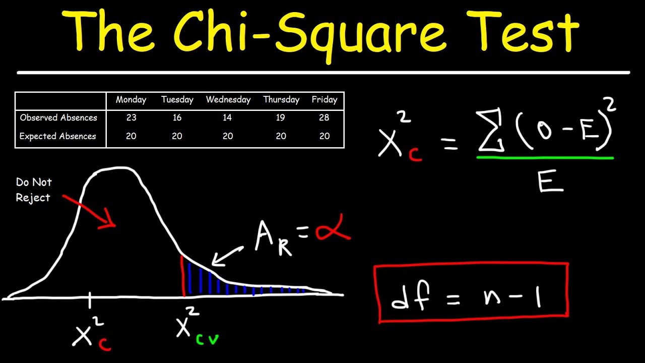
The chi-square statistic is calculated using the formula:
\[ \chi^2 = \sum \frac{(O_i - E_i)^2}{E_i} \]
Where:
- Oi = observed frequency
- Ei = expected frequency
Steps in Performing a Chi-Square Test
- Set Up Hypotheses: Define the null and alternative hypotheses.
- Calculate Expected Frequencies: Based on the marginal totals and overall sample size.
- Compute the Test Statistic: Use the chi-square formula to calculate the test statistic.
- Determine the P-value: Compare the chi-square statistic to the critical value from the chi-square distribution table.
- Conclusion: Decide whether to reject or fail to reject the null hypothesis based on the p-value.
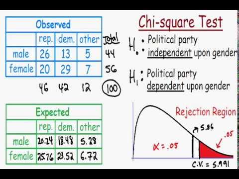
Example of a Chi-Square Test
Consider a study examining the relationship between gender and political party preference. The observed frequencies are tabulated, and the expected frequencies are calculated assuming independence. The test statistic is computed and compared to the critical value to determine if there is a significant association.
| Political Party | Male | Female | Total |
|---|---|---|---|
| Republican | 120 | 110 | 230 |
| Democrat | 90 | 95 | 185 |
| Independent | 40 | 45 | 85 |
| Total | 250 | 250 | 500 |
The expected frequencies are calculated and used to find the chi-square statistic. If the p-value is less than the significance level, we reject the null hypothesis, indicating a significant association between gender and political party preference.
:max_bytes(150000):strip_icc()/Chi-SquareStatistic_Final_4199464-7eebcd71a4bf4d9ca1a88d278845e674.jpg)
READ MORE:
Introduction to Chi-Square Test
The Chi-Square test is a statistical method used to examine the associations between categorical variables. This test is widely used in hypothesis testing to determine if there is a significant difference between the expected and observed frequencies in one or more categories.
There are two main types of Chi-Square tests: the Chi-Square Goodness of Fit test and the Chi-Square Test of Independence.
- Chi-Square Goodness of Fit Test: This test determines if a sample data matches a population with a specific distribution.
- Chi-Square Test of Independence: This test evaluates whether two categorical variables are independent of each other.
The general procedure for performing a Chi-Square test includes the following steps:
- State the Hypotheses: Formulate the null hypothesis (H0) and the alternative hypothesis (H1). The null hypothesis typically states that there is no association between the variables.
- Calculate Expected Frequencies: Compute the expected frequency for each category assuming the null hypothesis is true. The expected frequency is given by: \[ E = \frac{(\text{row total} \times \text{column total})}{\text{grand total}} \]
- Compute the Chi-Square Statistic: Use the formula: \[ \chi^2 = \sum \frac{(O - E)^2}{E} \] where \( O \) is the observed frequency and \( E \) is the expected frequency.
- Determine the Degrees of Freedom: Calculate the degrees of freedom as: \[ \text{df} = (r-1) \times (c-1) \] where \( r \) is the number of rows and \( c \) is the number of columns.
- Compare the Chi-Square Statistic to the Critical Value: Using a Chi-Square distribution table, find the critical value at the desired significance level (e.g., 0.05). If the computed Chi-Square statistic exceeds the critical value, reject the null hypothesis.
- Conclusion: Draw a conclusion based on the comparison. If the null hypothesis is rejected, it indicates a significant association between the variables.
The Chi-Square test is a powerful tool for analyzing categorical data and understanding relationships between variables in a dataset. It is essential in various fields such as social sciences, biology, and market research.
Null Hypothesis for Chi-Square Test
The null hypothesis for a chi-square test is a statement that assumes no association between the categorical variables being studied. It posits that any observed differences are due to random chance.
In a chi-square test, we calculate the chi-square statistic using the formula:
\[
\chi^2 = \sum \frac{{(O_i - E_i)^2}}{E_i}
\]
where:
- \( O_i \) is the observed frequency for each category.
- \( E_i \) is the expected frequency for each category, calculated based on the assumption that the null hypothesis is true.
To perform the chi-square test, follow these steps:
- Formulate the hypotheses:
- Null hypothesis (\( H_0 \)): The variables are independent (no association).
- Alternative hypothesis (\( H_1 \)): The variables are not independent (there is an association).
- Construct a contingency table of the observed frequencies.
- Calculate the expected frequencies for each cell in the table using the formula: \[ E_i = \frac{{\text{row total} \times \text{column total}}}{\text{grand total}} \]
- Compute the chi-square statistic using the observed and expected frequencies.
- Determine the degrees of freedom, which is given by: \[ \text{df} = (r - 1) \times (c - 1) \] where \( r \) is the number of rows and \( c \) is the number of columns.
- Compare the chi-square statistic to the critical value from the chi-square distribution table at the desired significance level (\( \alpha \)).
- Make a decision:
- If the chi-square statistic is greater than the critical value, reject the null hypothesis.
- If the chi-square statistic is less than or equal to the critical value, fail to reject the null hypothesis.
The chi-square test is widely used in research to test the relationship between categorical variables, helping researchers determine if their observed data deviate significantly from what was expected under the null hypothesis.
Chi-Square Test of Independence
The Chi-Square Test of Independence is a statistical method used to determine if there is a significant association between two categorical variables. This test is widely used in research to examine the relationship between variables such as gender and voting preferences, education level and employment status, or any other categorical data.
Here is a step-by-step guide to performing a Chi-Square Test of Independence:
-
Define the Hypotheses:
- Null Hypothesis (\(H_0\)): The two variables are independent.
- Alternative Hypothesis (\(H_1\)): The two variables are not independent (they are associated).
-
Construct the Contingency Table:
Collect and organize your data into a contingency table, which displays the frequency distribution of the variables.
-
Calculate the Expected Frequencies:
The expected frequency for each cell in the table is calculated using the formula:
\[
E = \frac{(\text{row total} \times \text{column total})}{\text{grand total}}
\] -
Compute the Chi-Square Statistic:
The test statistic is calculated using the formula:
\[
\chi^2 = \sum \frac{(O - E)^2}{E}
\]where \(O\) is the observed frequency and \(E\) is the expected frequency.
-
Determine the Degrees of Freedom:
The degrees of freedom (df) are calculated as:
\[
df = (r - 1) \times (c - 1)
\]where \(r\) is the number of rows and \(c\) is the number of columns in the contingency table.
-
Find the Critical Value and p-Value:
Using a Chi-Square distribution table or statistical software, find the critical value and p-value corresponding to the calculated \(\chi^2\) statistic and degrees of freedom.
-
Make a Decision:
Compare the p-value to your significance level (\(\alpha\)). If the p-value is less than \(\alpha\), reject the null hypothesis. This indicates that there is a significant association between the two variables.
The Chi-Square Test of Independence is a powerful tool for understanding relationships between categorical variables, helping researchers make data-driven decisions.
Steps to Perform a Chi-Square Test
The Chi-Square test is a statistical method used to determine if there is a significant association between categorical variables. The following are the steps to perform a Chi-Square test:
-
Define the Hypotheses:
- Null Hypothesis (\(H_0\)): There is no association between the variables.
- Alternative Hypothesis (\(H_1\)): There is an association between the variables.
-
Construct the Contingency Table: Organize the observed frequencies into a table.
Category 1 Category 2 Total Group 1 O11 O12 Row Total Group 2 O21 O22 Row Total Total Column Total Column Total Grand Total -
Calculate Expected Frequencies: Use the formula \(E_{ij} = \frac{\text{(Row Total) × (Column Total)}}{\text{Grand Total}}\) for each cell.
-
Compute the Chi-Square Statistic: Use the formula \(\chi^2 = \sum \frac{(O_{ij} - E_{ij})^2}{E_{ij}}\) where \(O_{ij}\) is the observed frequency and \(E_{ij}\) is the expected frequency.
-
Determine the Degrees of Freedom: Calculate degrees of freedom as \((r-1) \times (c-1)\), where \(r\) is the number of rows and \(c\) is the number of columns.
-
Find the Critical Value: Use a Chi-Square distribution table to find the critical value at your desired significance level.
-
Compare and Draw Conclusion: Compare the Chi-Square statistic to the critical value:
- If \(\chi^2\) is greater than the critical value, reject the null hypothesis.
- If \(\chi^2\) is less than or equal to the critical value, do not reject the null hypothesis.
Calculating Expected Frequencies
In a Chi-Square test, calculating the expected frequencies is a crucial step. The expected frequency for each cell in a contingency table is determined based on the assumption that there is no relationship between the variables, which is the null hypothesis.
The formula to calculate the expected frequency for each cell is:
\[ E_{ij} = \frac{(R_i \times C_j)}{N} \]
Where:
- \( E_{ij} \) is the expected frequency for cell \( i, j \).
- \( R_i \) is the total number of observations in row \( i \).
- \( C_j \) is the total number of observations in column \( j \).
- \( N \) is the grand total number of observations.
To illustrate this process, consider a 2x2 contingency table:
| Category 1 | Category 2 | Row Total | |
| Group A | O11 | O12 | R1 |
| Group B | O21 | O22 | R2 |
| Column Total | C1 | C2 | N |
The expected frequency for each cell can be calculated as follows:
For cell (1,1):
\[ E_{11} = \frac{(R_1 \times C_1)}{N} \]
For cell (1,2):
\[ E_{12} = \frac{(R_1 \times C_2)}{N} \]
For cell (2,1):
\[ E_{21} = \frac{(R_2 \times C_1)}{N} \]
For cell (2,2):
\[ E_{22} = \frac{(R_2 \times C_2)}{N} \]
After calculating the expected frequencies, you can compare them with the observed frequencies to determine if there is a significant difference, using the Chi-Square statistic.
Formulating the Null Hypothesis
The null hypothesis is a fundamental aspect of the Chi-Square test. It is a statement that suggests no relationship or effect between the variables under study. When formulating the null hypothesis for a Chi-Square test, follow these steps:
- Identify the Variables: Determine the categorical variables you want to test. For instance, if you are testing whether gender and political affiliation are independent, your variables are gender and political affiliation.
- State the Hypothesis of Independence: The null hypothesis for the Chi-Square test of independence posits that the two variables are not associated. It is typically formulated as:
\[ H_0: \text{The variables are independent} \]
For example, in testing if gender is independent of political party preference, the null hypothesis would be:
\[ H_0: \text{Gender and political party preference are independent} \]
- Collect Data: Gather the observed data into a contingency table where rows represent the categories of one variable and columns represent the categories of the other variable. Each cell in the table shows the frequency count of observations for each combination of categories.
- Calculate Expected Frequencies: Using the observed data, calculate the expected frequencies under the null hypothesis. The expected frequency for each cell is calculated using the formula:
\[ E_{ij} = \frac{( \text{Row Total} \times \text{Column Total} )}{\text{Grand Total}} \]
Where \( E_{ij} \) is the expected frequency for cell \( (i,j) \), Row Total is the sum of observations in the row, Column Total is the sum of observations in the column, and Grand Total is the total number of observations.
- Formulate the Alternative Hypothesis: The alternative hypothesis, denoted as \( H_1 \), suggests that there is a significant association between the variables. It is stated as:
\[ H_1: \text{The variables are dependent} \]
Continuing the earlier example, the alternative hypothesis would be:
\[ H_1: \text{Gender and political party preference are dependent} \]
- Assumptions Check: Ensure the data meets the assumptions required for the Chi-Square test. Each expected frequency should be at least 5 to ensure the validity of the test.
By following these steps, you can effectively formulate the null hypothesis for a Chi-Square test and proceed with the analysis to determine whether or not to reject the null hypothesis.
Test Statistic Calculation
The test statistic in a Chi-Square test is used to determine whether there is a significant difference between the observed and expected frequencies in a contingency table. The calculation involves several steps, which are detailed below:
- Set Up the Contingency Table: Organize your data into a contingency table that displays the frequency of occurrences for each combination of categories. For example, if you are studying the relationship between gender and political affiliation, your table might look like this:
Party A Party B Party C Male 30 50 20 Female 40 30 30 - Calculate the Expected Frequencies: For each cell in the table, calculate the expected frequency under the null hypothesis of independence using the formula:
\[ E_{ij} = \frac{(\text{Row Total}_i \times \text{Column Total}_j)}{\text{Grand Total}} \]
For instance, the expected frequency for the cell representing males and Party A would be calculated as:
\[ E_{11} = \frac{(\text{Total for Male} \times \text{Total for Party A})}{\text{Overall Total}} = \frac{(100 \times 70)}{200} = 35 \] - Compute the Chi-Square Statistic: Use the formula below to calculate the Chi-Square statistic (\( \chi^2 \)) by summing the squared differences between the observed (\( O \)) and expected (\( E \)) frequencies, divided by the expected frequencies for all cells in the table:
\[ \chi^2 = \sum \frac{(O_{ij} - E_{ij})^2}{E_{ij}} \]
Apply this calculation to each cell in the table. For example, for the cell representing males and Party A:
\[ \frac{(O_{11} - E_{11})^2}{E_{11}} = \frac{(30 - 35)^2}{35} = 0.714 \]Repeat this for all cells and sum these values to get the total Chi-Square statistic. Using the example table, it would be:
\[ \chi^2 = 0.714 + ... (\text{continue for each cell}) \] - Determine the Degrees of Freedom: Calculate the degrees of freedom for the test using the formula:
\[ \text{Degrees of Freedom} = (r - 1) \times (c - 1) \]
where \( r \) is the number of rows and \( c \) is the number of columns. For our example with 2 rows and 3 columns:
\[ (2 - 1) \times (3 - 1) = 2 \] - Compare to the Chi-Square Distribution: Finally, compare the calculated Chi-Square statistic to the critical value from the Chi-Square distribution table with the appropriate degrees of freedom and chosen significance level (e.g., 0.05). If the calculated statistic exceeds the critical value, you reject the null hypothesis.
By following these steps, you can accurately calculate the Chi-Square test statistic and determine the statistical significance of the observed data.
Decision Rule and Significance Level
Determining the outcome of a Chi-Square test involves setting a decision rule based on a pre-defined significance level. This process helps us decide whether to reject the null hypothesis. Follow these steps to understand how the decision rule and significance level work together:
- Choose the Significance Level (\( \alpha \)): The significance level is the probability threshold below which the null hypothesis will be rejected. Common choices for \( \alpha \) are 0.05, 0.01, and 0.10. The significance level represents the risk of rejecting the null hypothesis when it is actually true (Type I error). For example, if \( \alpha = 0.05 \), there is a 5% risk of concluding that there is an association between variables when there is none.
- Calculate the Degrees of Freedom: The degrees of freedom (df) for the Chi-Square test are calculated based on the number of categories in the variables being tested. For a contingency table, the formula is:
\[ \text{Degrees of Freedom} = (r - 1) \times (c - 1) \]
where \( r \) is the number of rows and \( c \) is the number of columns. For a 3x3 table:
\[ \text{df} = (3 - 1) \times (3 - 1) = 4 \] - Find the Critical Value: Using the Chi-Square distribution table, find the critical value corresponding to the chosen \( \alpha \) and calculated degrees of freedom. The critical value is the cutoff point beyond which the observed test statistic is considered statistically significant. For \( \alpha = 0.05 \) and 4 degrees of freedom, the critical value is approximately 9.488.
- State the Decision Rule: The decision rule determines whether to reject the null hypothesis based on the comparison of the test statistic to the critical value. The rule is:
- If \( \chi^2 \) (test statistic) > critical value, reject the null hypothesis (\( H_0 \)).
- If \( \chi^2 \) (test statistic) ≤ critical value, fail to reject the null hypothesis.
For instance, if our calculated \( \chi^2 \) is 12.0 and our critical value at \( \alpha = 0.05 \) and df = 4 is 9.488, we would reject \( H_0 \) because 12.0 > 9.488.
- Interpret the Results: Based on the decision rule, interpret the outcome of the test:
- Reject \( H_0 \): This suggests that there is sufficient evidence to conclude that there is a significant association between the variables.
- Fail to Reject \( H_0 \): This suggests that there is not enough evidence to conclude a significant association between the variables, and they are likely independent.
Using the example above, since our \( \chi^2 \) value (12.0) exceeds the critical value (9.488), we reject the null hypothesis and conclude that there is a significant association between the variables.
By carefully choosing the significance level and following the decision rule, you can make informed conclusions about the relationship between the variables in your Chi-Square test.

Interpreting the Results
Once you have performed a Chi-Square test and calculated the test statistic, the next step is to interpret the results. This involves understanding what the test statistic, p-value, and the decision rule imply about the relationship between the variables being studied. Follow these steps to interpret the Chi-Square test results:
- Examine the Test Statistic: The test statistic (\( \chi^2 \)) is calculated based on the observed and expected frequencies in your contingency table. A larger \( \chi^2 \) value indicates a greater discrepancy between the observed and expected frequencies, which may suggest a significant association between the variables. Compare your calculated \( \chi^2 \) value to the critical value from the Chi-Square distribution table for your chosen significance level and degrees of freedom.
- Check the P-Value: The p-value indicates the probability that the observed differences (or more extreme) could occur if the null hypothesis were true. Compare the p-value to your significance level (\( \alpha \)):
- If \( p \leq \alpha \), reject the null hypothesis (\( H_0 \)). This suggests that the observed frequencies are significantly different from the expected frequencies, implying an association between the variables.
- If \( p > \alpha \), fail to reject the null hypothesis. This suggests that there is not enough evidence to conclude that the observed frequencies are significantly different from the expected frequencies, implying no significant association between the variables.
- Interpret the Decision: Based on whether you rejected or failed to reject the null hypothesis, interpret what this means for your study:
- Reject \( H_0 \): If you reject the null hypothesis, it suggests that there is a statistically significant association between the variables. For example, if you tested the association between gender and political preference, rejecting \( H_0 \) would imply that gender is significantly associated with political preference.
- Fail to Reject \( H_0 \): If you fail to reject the null hypothesis, it suggests that there is no statistically significant association between the variables, and they are likely independent of each other. For the gender and political preference example, this would imply that there is no significant relationship between gender and political preference.
- Consider Practical Significance: Statistical significance does not always imply practical significance. Even if you find a significant association, consider the strength and practical implications of this relationship. Analyze the effect size and the real-world impact of the findings. In some cases, a statistically significant result might not be practically meaningful.
- Report the Results: Clearly report your findings, including the test statistic, degrees of freedom, p-value, and the conclusion about the null hypothesis. For example:
"The Chi-Square test of independence showed a significant association between gender and political preference, \( \chi^2(2, N = 200) = 10.83 \), \( p < 0.05 \). Therefore, we reject the null hypothesis and conclude that gender and political preference are significantly related."
- Visualize the Data: To enhance understanding, consider visualizing the data with bar charts or mosaic plots that show the observed frequencies and the differences from expected frequencies. This can provide a clear picture of how the variables are related.
By carefully interpreting the Chi-Square test results, you can draw meaningful conclusions about the relationships between your categorical variables and support your data-driven decision-making.
Examples of Chi-Square Test
The Chi-Square test is widely used in statistics to test hypotheses about the relationship between categorical variables. Here are a few detailed examples to illustrate how the Chi-Square test is applied in various scenarios:
- Example 1: Chi-Square Test of Independence
Imagine a researcher wants to examine whether there is an association between gender and preference for a type of movie genre (Action, Drama, or Comedy). The data is collected from a survey of 300 participants and organized into a contingency table:
Action Drama Comedy Male 60 30 50 Female 30 70 60 Other 10 50 40 The researcher performs a Chi-Square test of independence to determine if movie genre preference is independent of gender.
- Step 1: Calculate Expected Frequencies
The expected frequency for each cell is calculated as:
\[ E_{ij} = \frac{(\text{Row Total} \times \text{Column Total})}{\text{Grand Total}} \]For the cell (Male, Action), the expected frequency is:
\[ E_{11} = \frac{(140 \times 100)}{300} = 46.67 \] - Step 2: Compute the Chi-Square Statistic
Using the formula:
\[ \chi^2 = \sum \frac{(O_{ij} - E_{ij})^2}{E_{ij}} \]For the cell (Male, Action):
\[ \frac{(60 - 46.67)^2}{46.67} = 3.59 \]This calculation is repeated for each cell, and the sum gives the Chi-Square statistic.
- Step 3: Determine the Degrees of Freedom
Degrees of freedom are calculated as:
\[ (r - 1) \times (c - 1) = (3 - 1) \times (3 - 1) = 4 \] - Step 4: Compare to the Critical Value
Using a significance level of 0.05 and 4 degrees of freedom, the critical value from the Chi-Square distribution table is approximately 9.488. If the calculated Chi-Square statistic is greater than 9.488, the null hypothesis of independence is rejected.
Assuming our calculated Chi-Square statistic is 11.3, which is greater than 9.488, we reject the null hypothesis and conclude that there is a significant association between gender and movie genre preference.
- Step 1: Calculate Expected Frequencies
- Example 2: Chi-Square Goodness of Fit Test
A candy manufacturer wants to test if their candy production is equally distributed across four colors: red, blue, green, and yellow. A sample of 400 candies is taken, and the observed frequencies are recorded as follows:
Color Observed Frequency Red 90 Blue 110 Green 100 Yellow 100 The expected frequency for each color, if the distribution is equal, is:
\[ E = \frac{400}{4} = 100 \]- Step 1: Calculate the Chi-Square Statistic
Using the formula:
\[ \chi^2 = \sum \frac{(O_i - E_i)^2}{E_i} \]For the color Red:
\[ \frac{(90 - 100)^2}{100} = 1 \]Repeat for each color and sum the results to get the total Chi-Square statistic.
- Step 2: Determine the Degrees of Freedom
For a goodness of fit test, the degrees of freedom are:
\[ \text{df} = \text{Number of Categories} - 1 = 4 - 1 = 3 \] - Step 3: Compare to the Critical Value
With \( \alpha = 0.05 \) and 3 degrees of freedom, the critical value from the Chi-Square distribution table is approximately 7.815. If the calculated Chi-Square statistic exceeds this value, the null hypothesis that the distribution is equal is rejected.
Assuming our calculated Chi-Square statistic is 2.2, which is less than 7.815, we fail to reject the null hypothesis and conclude that the candies are equally distributed across the colors.
- Step 1: Calculate the Chi-Square Statistic
These examples illustrate the application of Chi-Square tests in evaluating associations between categorical variables and testing for equal distributions. By following these steps, you can apply the Chi-Square test to a variety of research questions involving categorical data.
Chi-Square Goodness of Fit Test
The Chi-Square Goodness of Fit Test is used to determine whether a sample data matches a population with a specific distribution. This test is often applied to see if a set of observed categorical data aligns with theoretical expectations. Here’s a step-by-step guide on how to perform and interpret the Chi-Square Goodness of Fit Test:
- Define the Hypotheses:
Formulate the null and alternative hypotheses. For the goodness of fit test, these are typically:
- Null Hypothesis (\( H_0 \)): The observed frequencies follow the expected distribution.
- Alternative Hypothesis (\( H_1 \)): The observed frequencies do not follow the expected distribution.
- Collect the Data:
Gather the observed frequencies from your sample data. Ensure that the data is categorized into appropriate groups or bins for analysis. For example, a candy company might categorize candies by color to test if they are produced in equal proportions.
- Determine the Expected Frequencies:
Calculate the expected frequencies for each category if the null hypothesis were true. The expected frequency (\( E_i \)) for each category is calculated using:
\[ E_i = N \times P_i \]Where \( N \) is the total number of observations and \( P_i \) is the probability of the category according to the hypothesized distribution. If you expect an equal distribution across four categories with 400 total observations, each category's expected frequency would be:
\[ E_i = \frac{400}{4} = 100 \] - Calculate the Chi-Square Statistic:
Use the formula to compute the Chi-Square statistic (\( \chi^2 \)):
\[ \chi^2 = \sum \frac{(O_i - E_i)^2}{E_i} \]Where \( O_i \) are the observed frequencies and \( E_i \) are the expected frequencies. Calculate this for each category and sum the results to get the total Chi-Square statistic. For example, if observed frequencies for four categories are [90, 110, 100, 100] and the expected frequencies are [100, 100, 100, 100], then:
\[ \chi^2 = \frac{(90 - 100)^2}{100} + \frac{(110 - 100)^2}{100} + \frac{(100 - 100)^2}{100} + \frac{(100 - 100)^2}{100} = 1 + 1 + 0 + 0 = 2 \] - Determine the Degrees of Freedom:
Calculate the degrees of freedom (df) for the test. For the goodness of fit test, degrees of freedom are calculated as:
\[ df = k - 1 \]Where \( k \) is the number of categories. For four categories:
\[ df = 4 - 1 = 3 \] - Find the Critical Value and Compare:
Refer to the Chi-Square distribution table to find the critical value for the chosen significance level (\( \alpha \)) and the degrees of freedom. For example, with \( \alpha = 0.05 \) and df = 3, the critical value is approximately 7.815.
Compare the calculated Chi-Square statistic to the critical value:
- If \( \chi^2 \) (calculated) > \( \chi^2 \) (critical), reject the null hypothesis.
- If \( \chi^2 \) (calculated) ≤ \( \chi^2 \) (critical), fail to reject the null hypothesis.
In our example, the calculated \( \chi^2 \) value is 2, which is less than 7.815, so we fail to reject the null hypothesis, suggesting that the distribution of candy colors matches the expected distribution.
- Interpret the Results:
Based on the comparison:
- Reject \( H_0 \): Conclude that the observed data does not fit the expected distribution.
- Fail to Reject \( H_0 \): Conclude that the observed data fits the expected distribution.
For example, if we reject \( H_0 \), it indicates that the production of candy colors is not equally distributed as hypothesized.
The Chi-Square Goodness of Fit Test provides a robust method for comparing observed data with a theoretical distribution, enabling researchers to validate or refute expected patterns in categorical data.
Applications in Real-World Scenarios
The Chi-Square test is a versatile statistical tool used to analyze the relationship between categorical variables in various real-world contexts. Below are several scenarios where the Chi-Square test is applied effectively:
- Market Research and Consumer Behavior:
Companies often use the Chi-Square test to understand consumer preferences and behaviors. For example, a retailer might want to know if the preference for a particular product category is independent of demographic factors like age or income. By collecting survey data and applying a Chi-Square test, they can assess whether there are significant differences in product preferences among different demographic groups.
Example:
- Scenario: A company surveys 200 customers to see if there is a significant difference in the preference for three types of products (Product A, Product B, Product C) across different age groups (18-25, 26-35, 36-45).
- Application: By organizing the data into a contingency table and performing a Chi-Square test of independence, the company can determine if age group significantly influences product preference.
- Healthcare and Medicine:
In healthcare, the Chi-Square test helps in studying the association between patient characteristics and health outcomes. For example, researchers might investigate whether the incidence of a certain disease is related to lifestyle factors such as smoking or diet.
Example:
- Scenario: A study examines whether the occurrence of a particular health condition (e.g., diabetes) is independent of lifestyle choices (e.g., smoking status: smoker, non-smoker).
- Application: Using a Chi-Square test, researchers can determine if there is a significant association between smoking status and the incidence of diabetes among the study participants.
- Education and Academic Research:
Educational researchers frequently use the Chi-Square test to explore the relationship between students' demographics and their academic performance. For instance, they might assess if student performance in a subject is associated with their socioeconomic status.
Example:
- Scenario: An educational study investigates whether the success rate in passing a standardized test is associated with the type of school attended (public, private, charter).
- Application: By performing a Chi-Square test of independence, researchers can analyze if there are statistically significant differences in test pass rates across different types of schools.
- Social Science and Public Policy:
Social scientists use the Chi-Square test to study the relationships between societal factors and behaviors. For instance, they might examine whether voting patterns in an election are independent of gender or education level.
Example:
- Scenario: A public policy analyst wants to understand if the support for different political parties varies by educational attainment (high school, undergraduate, graduate).
- Application: By applying a Chi-Square test to survey data, the analyst can determine if there is a significant relationship between education level and political party preference.
- Quality Control and Manufacturing:
Manufacturers use the Chi-Square test to ensure product quality and consistency. For example, they might test if the defect rates of products are independent of the manufacturing shifts (morning, afternoon, night).
Example:
- Scenario: A factory collects data on defective items produced during different shifts and wants to determine if defect rates are significantly different between shifts.
- Application: By using a Chi-Square test of independence, the quality control team can analyze whether the time of shift impacts the defect rate, helping them identify potential issues in production processes.
- Environmental Science:
Environmental researchers apply the Chi-Square test to study the distribution of species or environmental conditions across different regions or habitats. For instance, they might examine if the distribution of a particular plant species is independent of soil type.
Example:
- Scenario: An ecologist wants to determine if the distribution of a certain plant species varies significantly with different soil types (sandy, clay, loamy).
- Application: By organizing the data into a contingency table and performing a Chi-Square test, the ecologist can assess whether the presence of the plant species is significantly associated with the soil type.
These examples illustrate how the Chi-Square test can be employed across various fields to test hypotheses about the relationships between categorical variables, providing valuable insights for decision-making and research.
Software Tools for Chi-Square Test
Several software tools are available to perform Chi-Square tests efficiently, providing researchers and analysts with user-friendly interfaces and robust statistical capabilities. Here are some widely used software tools for conducting Chi-Square tests, along with a brief overview of their features and how to use them:
- Microsoft Excel:
Excel is a versatile tool that includes functions for performing Chi-Square tests, making it accessible for many users.
- How to Use:
- Input your observed and expected frequency data into a spreadsheet.
- Use the
CHISQ.TESTfunction to compute the Chi-Square statistic and p-value. - Alternatively, create a contingency table and use Excel’s Data Analysis Toolpak to perform the Chi-Square test of independence.
- Advantages: Widely available, easy to use for basic analysis, and does not require advanced statistical knowledge.
- How to Use:
- IBM SPSS Statistics:
SPSS is a powerful statistical software widely used in social sciences and business research.
- How to Use:
- Load your dataset into SPSS.
- Navigate to Analyze > Descriptive Statistics > Crosstabs.
- Select the variables you want to test and check the Chi-Square option under Statistics.
- Run the analysis to get detailed output including Chi-Square statistic, degrees of freedom, and p-value.
- Advantages: Provides comprehensive statistical analysis, including detailed outputs and options for different types of Chi-Square tests.
- How to Use:
- R Programming Language:
R is an open-source statistical programming language that offers extensive packages for performing Chi-Square tests.
- How to Use:
- Install R and open an R script or console.
- Load your data into R, typically using
read.csv()or similar functions. - Use the
chisq.test()function to perform the Chi-Square test. For example,chisq.test(observed, expected)for a goodness of fit test, orchisq.test(table)for a test of independence. - Review the output which includes the Chi-Square statistic, p-value, and degrees of freedom.
- Advantages: Highly flexible and customizable for complex analyses, with strong community support and extensive documentation.
- How to Use:
- Python with SciPy Library:
Python, particularly with the SciPy library, is a popular choice for statistical analysis, including Chi-Square tests.
- How to Use:
- Install Python and the necessary libraries, including
scipyandpandas. - Load your data into a DataFrame using
pandas. - Use
scipy.stats.chisquare()for the goodness of fit test, orscipy.stats.chi2_contingency()for the test of independence. - Interpret the results which include the Chi-Square statistic, p-value, and degrees of freedom.
- Install Python and the necessary libraries, including
- Advantages: Great for integrating statistical analysis with other data processing and machine learning tasks, with powerful data manipulation capabilities.
- How to Use:
- Statistical Software for Data Science (Stata):
Stata is a robust software used in academia and research for statistical analysis.
- How to Use:
- Load your dataset into Stata.
- Use the
tabulatecommand for contingency tables, followed by thechi2option to perform the Chi-Square test of independence. - For the goodness of fit test, use the
bitestcommand. - Examine the detailed output provided, which includes Chi-Square statistic and p-value.
- Advantages: Known for its ease of use and extensive statistical capabilities, particularly popular in econometrics and social sciences.
- How to Use:
These tools provide a range of options for conducting Chi-Square tests, from basic spreadsheet software like Excel to more advanced statistical programs like SPSS, R, Python, and Stata. Selecting the right tool depends on your specific needs, data complexity, and familiarity with the software.
Common Pitfalls and Considerations
While the Chi-Square test is a powerful tool for statistical analysis, it is essential to be aware of certain pitfalls and considerations to ensure accurate and meaningful results. Here are some common challenges and key points to keep in mind:
- Sample Size Requirements:
The Chi-Square test requires an adequate sample size to provide reliable results. Small sample sizes can lead to inaccurate conclusions due to low statistical power.
- It is generally recommended that the expected frequency in each cell of a contingency table be at least 5.
- If many expected frequencies are below this threshold, consider combining categories or using alternative tests like Fisher's Exact Test for smaller samples.
- Expected Frequencies:
Chi-Square tests rely on the comparison between observed and expected frequencies. Accurate calculation of expected frequencies is crucial for valid results.
- Ensure that expected frequencies are calculated correctly based on the null hypothesis assumptions.
- Misinterpreting or incorrectly computing these frequencies can lead to misleading conclusions.
- Independence Assumption:
One of the key assumptions of the Chi-Square test is that the observations are independent of each other.
- If the data violates this assumption (e.g., paired or repeated measurements), the test results will not be valid.
- In cases of dependent samples, consider using tests designed for such data structures, like the McNemar's test for paired nominal data.
- Cell Counts:
Chi-Square tests are sensitive to the distribution of counts in contingency tables.
- A high proportion of low cell counts (especially zeroes) can invalidate the test results.
- Large tables with many cells having low expected counts may require combining categories or choosing alternative methods.
- Interpretation of Results:
Interpreting the results of a Chi-Square test goes beyond simply checking if the p-value is below a significance threshold.
- Always consider the context and practical significance of the findings, not just the statistical significance.
- A significant Chi-Square result indicates a departure from the null hypothesis, but further investigation is needed to understand the nature and magnitude of the association.
- Multiple Comparisons:
When conducting multiple Chi-Square tests, the risk of Type I errors increases, meaning that you are more likely to find a significant result by chance.
- Consider using a correction method, such as the Bonferroni correction, to adjust for multiple comparisons and control the family-wise error rate.
- Be cautious about drawing conclusions from multiple tests without appropriate adjustments.
- Data Type and Test Selection:
The Chi-Square test is designed for categorical data. Using it inappropriately for continuous data can lead to incorrect results.
- If you have continuous data, consider using alternative statistical tests like ANOVA or t-tests, depending on the study design and hypotheses.
- Ensure the data type matches the assumptions of the Chi-Square test to maintain the validity of your analysis.
- Assumption of Homogeneity:
In a Chi-Square test of independence, it is assumed that the distribution of counts is homogeneous across the categories.
- If the data shows significant heterogeneity, the test results may not be valid.
- Consider alternative approaches or transformations if heterogeneity is a concern.
By being aware of these pitfalls and considerations, you can enhance the reliability and interpretability of your Chi-Square test results. Careful planning and understanding of the test's assumptions and limitations are crucial for effective statistical analysis.
Conclusion and Further Reading
The Chi-Square test is a versatile and widely used statistical method for examining the association between categorical variables. Whether you are testing for independence or assessing the goodness of fit, understanding the nuances of the Chi-Square test allows for robust and meaningful data analysis. Here are the key takeaways from our discussion:
- Understanding the Null Hypothesis:
The null hypothesis is a fundamental aspect of the Chi-Square test, asserting that there is no significant association between the observed categorical variables. Properly defining and testing this hypothesis is crucial to the integrity of the test.
- Test Statistic Calculation:
The Chi-Square statistic quantifies the divergence between observed and expected frequencies. Calculating this statistic accurately helps in assessing the validity of the null hypothesis.
- Decision Rule and Significance Level:
Setting an appropriate significance level and understanding the decision rule for rejecting or failing to reject the null hypothesis is essential for correct interpretation of the test results.
- Interpreting the Results:
Interpreting the Chi-Square test results involves examining the p-value and the context of the research question. A significant result suggests a relationship between variables, but the practical significance should also be considered.
- Common Pitfalls:
Avoiding common pitfalls such as small sample sizes, low expected frequencies, and misinterpretation of results is vital for the reliability of the test.
- Applications in Real-World Scenarios:
The Chi-Square test is used in various fields, from social sciences to business analytics, to test hypotheses about categorical data.
- Software Tools:
Several software tools, including Excel, SPSS, R, and Python, offer robust functionalities for conducting Chi-Square tests, making the process accessible and efficient for researchers and analysts.
As you delve deeper into the use of Chi-Square tests, consider exploring additional resources and readings to expand your knowledge and application skills:
- Textbooks:
- “Introduction to the Practice of Statistics” by Moore, McCabe, and Craig – Offers a comprehensive overview of statistical methods, including Chi-Square tests.
- “Statistics for Business and Economics” by Anderson, Sweeney, and Williams – Provides practical applications of Chi-Square tests in business and economics.
- Online Courses:
- – Covers the basics of hypothesis testing and includes practical applications of Chi-Square tests.
- – Provides a broader understanding of statistical principles, including Chi-Square tests.
- Research Articles:
- – A detailed article explaining the Chi-Square test, its applications, and interpretations.
- – Discusses the use of Chi-Square tests in business research settings.
By leveraging these resources, you can further enhance your understanding and application of the Chi-Square test, ensuring accurate and insightful data analysis in your projects.
Tìm hiểu về kiểm định Chi-Square trong thống kê. Hướng dẫn chi tiết cách thực hiện và giải thích về giả thuyết không cho kiểm định Chi-Square.
Kiểm Định Chi-Square
READ MORE:
Khám phá thống kê Chi-Square cho kiểm định giả thuyết trong khóa học Thống Kê AP của Khan Academy. Hướng dẫn chi tiết và giải thích về giả thuyết không cho kiểm định Chi-Square.
Thống Kê Chi-Square Cho Kiểm Định Giả Thuyết | Thống Kê AP | Khan Academy