Topic null hypothesis for chi square goodness of fit: The null hypothesis for chi-square goodness of fit is essential in statistical analysis, providing a foundation for determining if observed data fits an expected distribution. This comprehensive guide will help you understand the concept, assumptions, and steps involved in performing the chi-square goodness of fit test, making your data analysis more robust and insightful.
Table of Content
- Chi-Square Goodness of Fit Test
- Introduction to Chi-Square Goodness of Fit
- Defining the Null Hypothesis
- Assumptions of the Chi-Square Goodness of Fit Test
- Formulating the Null and Alternative Hypotheses
- Steps to Perform the Chi-Square Goodness of Fit Test
- Calculating the Chi-Square Statistic
- Interpreting the Results
- Examples and Applications
- Common Mistakes and Misconceptions
- FAQs on Chi-Square Goodness of Fit
- Conclusion
- YOUTUBE: Kiểm định chi bình phương của Pearson (phù hợp với mô hình) | Xác suất và Thống kê | Khan Academy
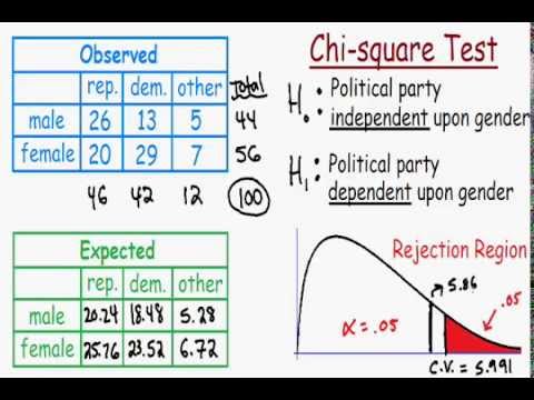
Chi-Square Goodness of Fit Test
The Chi-Square Goodness of Fit Test is a statistical hypothesis test used to determine whether a sample data matches a population with a specific distribution. This test is particularly useful for categorical data.
Null Hypothesis
The null hypothesis (\( H_0 \)) for the chi-square goodness of fit test states that the sample data fits the expected distribution. This can be mathematically represented as:
\[ H_0: \text{The data follows the expected distribution} \]
Alternative Hypothesis
The alternative hypothesis (\( H_a \)) indicates that the sample data does not fit the expected distribution:
\[ H_a: \text{The data does not follow the expected distribution} \]
Test Statistic
The test statistic for the chi-square goodness of fit test is calculated using the following formula:
\[ \chi^2 = \sum \frac{(O_i - E_i)^2}{E_i} \]
where:
- \( O_i \) = Observed frequency
- \( E_i \) = Expected frequency
Steps to Perform the Test
- State the hypotheses: Define the null and alternative hypotheses.
- Calculate the expected frequencies: Determine the expected frequencies based on the hypothesized distribution.
- Compute the test statistic: Use the chi-square formula to calculate the test statistic.
- Determine the degrees of freedom: The degrees of freedom for this test are calculated as \( df = k - 1 \), where \( k \) is the number of categories.
- Find the critical value: Use the chi-square distribution table to find the critical value at the desired significance level.
- Make a decision: Compare the test statistic to the critical value to determine whether to reject the null hypothesis.
Example
Suppose we want to test if a die is fair. The expected distribution for a fair six-sided die is that each side will occur with equal probability (1/6).
| Side of Die | Observed Frequency (\( O_i \)) | Expected Frequency (\( E_i \)) |
|---|---|---|
| 1 | 8 | 10 |
| 2 | 12 | 10 |
| 3 | 11 | 10 |
| 4 | 9 | 10 |
| 5 | 10 | 10 |
| 6 | 10 | 10 |
Calculate the test statistic:
\[ \chi^2 = \frac{(8-10)^2}{10} + \frac{(12-10)^2}{10} + \frac{(11-10)^2}{10} + \frac{(9-10)^2}{10} + \frac{(10-10)^2}{10} + \frac{(10-10)^2}{10} \]
\[ \chi^2 = \frac{4}{10} + \frac{4}{10} + \frac{1}{10} + \frac{1}{10} + \frac{0}{10} + \frac{0}{10} \]
\[ \chi^2 = 1 \]
With 5 degrees of freedom (df = 6 - 1) and a significance level of 0.05, we compare the calculated chi-square value to the critical value from the chi-square distribution table. If the chi-square value is less than the critical value, we fail to reject the null hypothesis, suggesting that the die is fair.
READ MORE:
Introduction to Chi-Square Goodness of Fit
The chi-square goodness of fit test is a statistical method used to determine how well observed data fits an expected distribution. This test compares the observed frequencies of a categorical dataset with the expected frequencies derived from a specific hypothesis. It is widely used in various fields, including biology, marketing, and social sciences, to test the validity of theoretical distributions.
In a chi-square goodness of fit test, the null hypothesis (\(H_0\)) states that there is no significant difference between the observed and expected frequencies. The alternative hypothesis (\(H_A\)) suggests that a significant difference exists. The test uses the chi-square statistic, calculated as follows:
\[ \chi^2 = \sum \frac{(O_i - E_i)^2}{E_i} \]
where:
- \(O_i\) represents the observed frequency of category \(i\)
- \(E_i\) represents the expected frequency of category \(i\)
Steps to perform the chi-square goodness of fit test:
- State the hypotheses: Formulate the null and alternative hypotheses.
- Calculate the expected frequencies: Determine the expected frequencies based on the hypothesized distribution.
- Compute the chi-square statistic: Use the formula to calculate the chi-square value.
- Determine the degrees of freedom: Calculate the degrees of freedom as \(df = k - 1\), where \(k\) is the number of categories.
- Find the critical value: Refer to the chi-square distribution table to find the critical value at the desired significance level.
- Compare and conclude: Compare the calculated chi-square statistic with the critical value to determine whether to reject or fail to reject the null hypothesis.
By following these steps, you can effectively use the chi-square goodness of fit test to assess how well your observed data matches the expected distribution, providing valuable insights into your research or analysis.
Defining the Null Hypothesis
The null hypothesis (\(H_0\)) in the context of the chi-square goodness of fit test is a statement that there is no significant difference between the observed frequencies and the expected frequencies of a categorical dataset. It serves as a baseline assumption that any deviations between observed and expected data are due to random chance.
The null hypothesis is formulated as:
\[ H_0: O_i = E_i \]
where:
- \(O_i\) represents the observed frequency of category \(i\)
- \(E_i\) represents the expected frequency of category \(i\)
Steps to define and test the null hypothesis:
- Identify the categories: Determine the categories for which the frequencies will be compared.
- Collect observed data: Gather the observed frequencies for each category.
- Determine the expected frequencies: Calculate the expected frequencies based on the hypothesized distribution or theoretical model.
- Formulate the null hypothesis: State that the observed frequencies are equal to the expected frequencies for all categories.
- Perform the chi-square test: Use the chi-square statistic to compare the observed and expected frequencies.
- Analyze the results: Compare the calculated chi-square statistic to the critical value from the chi-square distribution table to determine if the null hypothesis can be rejected.
By clearly defining the null hypothesis, researchers can objectively test whether their observed data significantly deviates from what was expected, allowing for a more rigorous and reliable analysis of categorical data.
Assumptions of the Chi-Square Goodness of Fit Test
The chi-square goodness of fit test relies on several key assumptions to ensure the validity and accuracy of its results. These assumptions must be met to properly apply the test and interpret the outcomes. The main assumptions are as follows:
- Random Sampling: The data should be collected through a random sampling method, ensuring that each member of the population has an equal chance of being included in the sample.
- Independence of Observations: Each observation must be independent of others, meaning the occurrence of one event does not influence the occurrence of another.
- Expected Frequency: The expected frequency for each category should be at least 5. If the expected frequencies are too low, the chi-square test may not be valid. This ensures that the test has enough power to detect differences.
- Mutually Exclusive Categories: The categories must be mutually exclusive, meaning that each observation can belong to only one category. There should be no overlap between categories.
- Large Sample Size: While not a strict requirement, a larger sample size generally provides more reliable results, reducing the margin of error in the test.
Meeting these assumptions is crucial for the chi-square goodness of fit test to provide accurate and reliable results. By ensuring that your data adheres to these conditions, you can confidently use the chi-square test to evaluate the goodness of fit between observed and expected frequencies.
Formulating the Null and Alternative Hypotheses
Formulating the null and alternative hypotheses is a critical step in the chi-square goodness of fit test. These hypotheses provide a clear statement of what you are testing and set the foundation for the statistical analysis. Here's how to formulate these hypotheses step-by-step:
- Identify the Categories: Determine the categories for which you will compare the observed and expected frequencies.
- State the Null Hypothesis (\(H_0\)): The null hypothesis asserts that there is no significant difference between the observed and expected frequencies. It can be formulated as:
\[ H_0: O_i = E_i \]- \(O_i\) represents the observed frequency for category \(i\)
- \(E_i\) represents the expected frequency for category \(i\)
- State the Alternative Hypothesis (\(H_A\)): The alternative hypothesis suggests that there is a significant difference between the observed and expected frequencies. It can be formulated as:
\[ H_A: O_i \neq E_i \]- \(O_i\) represents the observed frequency for category \(i\)
- \(E_i\) represents the expected frequency for category \(i\)
- Specify the Level of Significance: Choose a significance level (commonly denoted as \(\alpha\)) such as 0.05 or 0.01. This level determines the threshold for rejecting the null hypothesis.
- Collect and Analyze Data: Gather the observed data and calculate the expected frequencies based on the theoretical distribution or model.
- Perform the Chi-Square Test: Calculate the chi-square statistic using the formula:
\[ \chi^2 = \sum \frac{(O_i - E_i)^2}{E_i} \]- \(O_i\) represents the observed frequency for category \(i\)
- \(E_i\) represents the expected frequency for category \(i\)
- Compare to the Critical Value: Compare the calculated chi-square statistic to the critical value from the chi-square distribution table based on the chosen significance level and degrees of freedom.
- Draw Conclusions: If the chi-square statistic exceeds the critical value, reject the null hypothesis in favor of the alternative hypothesis. If it does not, fail to reject the null hypothesis.
By carefully formulating the null and alternative hypotheses, researchers can systematically test their data and draw meaningful conclusions about the relationship between observed and expected frequencies.
Steps to Perform the Chi-Square Goodness of Fit Test
The chi-square goodness of fit test is used to determine how well observed data matches an expected distribution. Follow these detailed steps to perform the test:
- Formulate the Hypotheses:
- Null Hypothesis (\(H_0\)): The observed frequencies are equal to the expected frequencies.
- Alternative Hypothesis (\(H_A\)): The observed frequencies are not equal to the expected frequencies.
- Collect the Data: Gather the observed frequencies for each category in your data set.
- Determine the Expected Frequencies: Calculate the expected frequencies based on a theoretical distribution or historical data. The expected frequency for each category can be calculated as:
\[ E_i = N \cdot p_i \]- \(E_i\) is the expected frequency for category \(i\)
- \(N\) is the total number of observations
- \(p_i\) is the probability of category \(i\) under the null hypothesis
- Calculate the Chi-Square Statistic: Use the formula:
\[ \chi^2 = \sum \frac{(O_i - E_i)^2}{E_i} \]- \(O_i\) is the observed frequency for category \(i\)
- \(E_i\) is the expected frequency for category \(i\)
- Determine the Degrees of Freedom: Calculate the degrees of freedom as:
\[ df = k - 1 \]- \(df\) is the degrees of freedom
- \(k\) is the number of categories
- Find the Critical Value: Refer to the chi-square distribution table to find the critical value based on your significance level (\(\alpha\)) and degrees of freedom.
- Compare the Calculated Chi-Square Statistic to the Critical Value: If the chi-square statistic exceeds the critical value, reject the null hypothesis. Otherwise, fail to reject the null hypothesis.
- Draw Conclusions: Interpret the results of your test in the context of your research question. If you rejected the null hypothesis, there is evidence to suggest that the observed data does not fit the expected distribution. If you failed to reject the null hypothesis, there is not enough evidence to suggest a significant difference.
By following these steps, you can effectively perform the chi-square goodness of fit test and determine the relationship between your observed data and the expected distribution.
Calculating the Chi-Square Statistic
Calculating the chi-square statistic is a crucial step in the chi-square goodness of fit test. This statistic helps determine how well the observed frequencies match the expected frequencies under the null hypothesis. Follow these detailed steps to calculate the chi-square statistic:
- Gather Observed Frequencies (\(O_i\)): Collect the observed frequencies for each category in your dataset.
- Calculate Expected Frequencies (\(E_i\)): Determine the expected frequencies based on the theoretical distribution or historical data. The expected frequency for each category can be calculated as:
\[ E_i = N \cdot p_i \]- \(E_i\) is the expected frequency for category \(i\)
- \(N\) is the total number of observations
- \(p_i\) is the probability of category \(i\) under the null hypothesis
- Apply the Chi-Square Formula: Use the chi-square formula to calculate the statistic:
\[ \chi^2 = \sum \frac{(O_i - E_i)^2}{E_i} \]- \(O_i\) is the observed frequency for category \(i\)
- \(E_i\) is the expected frequency for category \(i\)
- Calculate Each Component: For each category, compute the value of \(\frac{(O_i - E_i)^2}{E_i}\). Sum these values to obtain the chi-square statistic.
Example:
Category Observed Frequency (\(O_i\)) Expected Frequency (\(E_i\)) Component (\(\frac{(O_i - E_i)^2}{E_i}\)) A 50 45 0.56 B 30 35 0.71 C 20 20 0 Sum of components: \(0.56 + 0.71 + 0 = 1.27\)
- Interpret the Chi-Square Statistic: Compare the calculated chi-square statistic to the critical value from the chi-square distribution table, based on your chosen significance level and degrees of freedom.
By following these steps, you can accurately calculate the chi-square statistic, which will help you determine if there is a significant difference between the observed and expected frequencies in your data.
Interpreting the Results
Interpreting the results of a chi-square goodness of fit test involves comparing the calculated chi-square statistic to a critical value from the chi-square distribution table. This process helps determine whether to reject the null hypothesis. Follow these steps for a detailed interpretation:
- Calculate the Degrees of Freedom: Determine the degrees of freedom (\(df\)) for the test using the formula:
\[ df = k - 1 \]- \(df\) is the degrees of freedom
- \(k\) is the number of categories
- Choose the Significance Level: Select a significance level (\(\alpha\)), commonly 0.05 or 0.01, which defines the threshold for rejecting the null hypothesis.
- Find the Critical Value: Use the chi-square distribution table to find the critical value corresponding to the chosen significance level and degrees of freedom.
- Compare the Chi-Square Statistic to the Critical Value: Evaluate whether the calculated chi-square statistic exceeds the critical value:
- If \(\chi^2\) > Critical Value: Reject the null hypothesis (\(H_0\)). This indicates that there is a significant difference between the observed and expected frequencies.
- If \(\chi^2\) ≤ Critical Value: Fail to reject the null hypothesis (\(H_0\)). This suggests that any differences between the observed and expected frequencies are due to random chance.
- Draw Conclusions: Summarize the findings based on the comparison:
- Rejecting \(H_0\): There is evidence to suggest that the observed data does not fit the expected distribution. Further investigation may be needed to understand the cause of the discrepancy.
- Failing to Reject \(H_0\): There is no sufficient evidence to conclude a significant difference between the observed and expected frequencies. The observed data fits the expected distribution well.
- Report the Results: Clearly communicate the test results in your analysis. Include the chi-square statistic, degrees of freedom, significance level, and conclusion. For example:
\[ \chi^2 (df) = \text{value}, p \text{value} = \text{value} \]Example: \( \chi^2 (2) = 5.99, p = 0.05 \)
By following these steps, you can accurately interpret the results of the chi-square goodness of fit test and determine the relationship between the observed and expected frequencies in your data.
Examples and Applications
The chi-square goodness of fit test is widely used in various fields to determine if an observed frequency distribution matches an expected distribution. Here are some detailed examples and applications of the chi-square goodness of fit test:
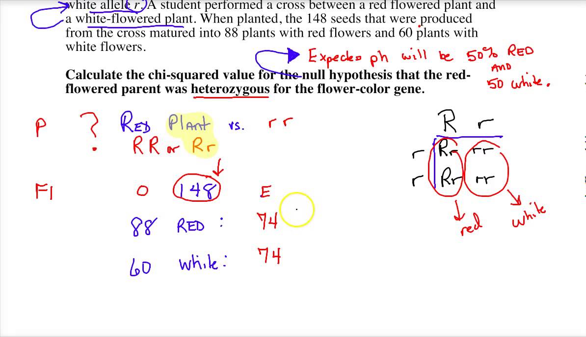
Example 1: Genetic Inheritance
Suppose a biologist wants to test if the observed frequencies of different phenotypes in a population of plants follow Mendelian inheritance ratios (3:1). The steps would be:
- Formulate the Hypotheses:
- Null Hypothesis (\(H_0\)): The observed frequencies follow a 3:1 ratio.
- Alternative Hypothesis (\(H_A\)): The observed frequencies do not follow a 3:1 ratio.
- Collect Data: Observe the number of plants with each phenotype. For instance, 75 tall and 25 short plants in a sample of 100.
- Calculate Expected Frequencies:
- Expected frequency of tall plants: \(E_1 = 0.75 \times 100 = 75\)
- Expected frequency of short plants: \(E_2 = 0.25 \times 100 = 25\)
- Calculate the Chi-Square Statistic:
\[
\chi^2 = \sum \frac{(O_i - E_i)^2}{E_i} = \frac{(75 - 75)^2}{75} + \frac{(25 - 25)^2}{25} = 0
\] - Compare to Critical Value: With \(df = 1\) and \(\alpha = 0.05\), the critical value from the chi-square table is 3.84. Since 0 < 3.84, we fail to reject \(H_0\).
- Conclusion: The observed frequencies follow the expected 3:1 Mendelian ratio.
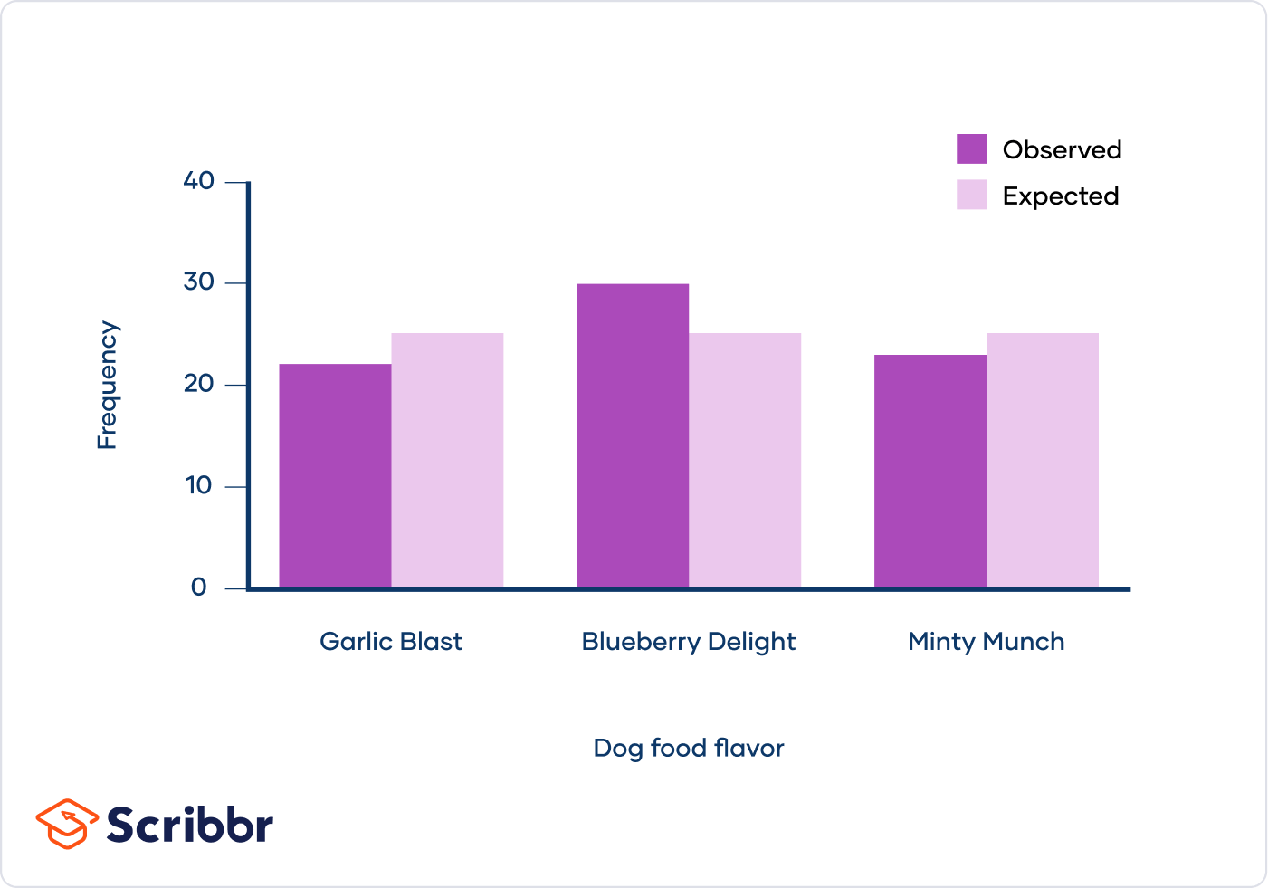
Example 2: Marketing Survey
A company wants to know if customer preferences for three products (A, B, C) are uniformly distributed. They survey 90 customers and find 20 prefer A, 30 prefer B, and 40 prefer C. The steps are:
- Formulate the Hypotheses:
- Null Hypothesis (\(H_0\)): Customer preferences are uniformly distributed across products.
- Alternative Hypothesis (\(H_A\)): Customer preferences are not uniformly distributed.
- Collect Data: Record the number of preferences for each product: A=20, B=30, C=40.
- Calculate Expected Frequencies:
- Expected frequency for each product: \(E_i = \frac{90}{3} = 30\)
- Calculate the Chi-Square Statistic:
\[
\chi^2 = \frac{(20 - 30)^2}{30} + \frac{(30 - 30)^2}{30} + \frac{(40 - 30)^2}{30} = \frac{100}{30} + 0 + \frac{100}{30} = 6.67
\] - Compare to Critical Value: With \(df = 2\) and \(\alpha = 0.05\), the critical value is 5.99. Since 6.67 > 5.99, we reject \(H_0\).
- Conclusion: Customer preferences are not uniformly distributed across the three products.
Applications
- Biology: Testing genetic inheritance patterns, ecological studies on species distribution.
- Marketing: Analyzing consumer preferences, product acceptance testing.
- Education: Examining the distribution of test scores, demographic studies of student populations.
- Healthcare: Studying the distribution of diseases, effectiveness of treatment methods.
- Social Sciences: Survey analysis, studying voting patterns, and population studies.
These examples and applications illustrate how the chi-square goodness of fit test can be used to test hypotheses and analyze categorical data across various fields.
Common Mistakes and Misconceptions
The Chi-Square Goodness of Fit test is a powerful tool for statistical analysis, but it is important to be aware of common mistakes and misconceptions to ensure accurate and valid results. Below are some of the most frequently encountered issues:
- Misinterpreting the Null Hypothesis: A common misconception is that the null hypothesis (H0) in the Chi-Square Goodness of Fit test implies that all observed frequencies must exactly match the expected frequencies. In reality, H0 suggests that any differences between observed and expected frequencies are due to random chance.
- Ignoring Sample Size Requirements: The test requires a sufficiently large sample size for the chi-square approximation to be valid. Small sample sizes can lead to inaccurate results. A rule of thumb is that the expected frequency for each category should be at least 5.
- Incorrectly Calculating Expected Frequencies: Errors in calculating expected frequencies can lead to incorrect chi-square statistics. Ensure that expected frequencies are computed based on the theoretical distribution under the null hypothesis.
- Combining Categories: Sometimes categories are combined to meet the minimum expected frequency requirement. However, this can distort the analysis. Combine categories only if it makes sense logically and does not obscure important differences.
- Overlooking Assumptions: The test assumes that the observations are independent of each other and that the data is categorical. Violating these assumptions can lead to invalid results.
- Misunderstanding P-values: A common mistake is to interpret the p-value as the probability that the null hypothesis is true. Instead, the p-value indicates the probability of obtaining a test statistic at least as extreme as the one observed, assuming that the null hypothesis is true.
- Neglecting Post-hoc Tests: When the null hypothesis is rejected, it is important to conduct post-hoc tests to determine which categories differ significantly. Simply knowing that there is a difference is not enough; identifying where the differences lie is crucial.
FAQs on Chi-Square Goodness of Fit
-
What is the null hypothesis for the Chi-Square Goodness of Fit test?
The null hypothesis (\(H_0\)) states that the observed frequencies in each category match the expected frequencies, meaning the data follows a specific distribution. For example, if you are testing if dice rolls are fair, the null hypothesis would be that each number appears with equal frequency.
-
How do I calculate the Chi-Square statistic?
The Chi-Square statistic is calculated using the formula:
\[\chi^2 = \sum \frac{(O - E)^2}{E}\]where \(O\) represents the observed frequency and \(E\) represents the expected frequency for each category. Sum this value across all categories to get the Chi-Square statistic.
-
What are the assumptions of the Chi-Square Goodness of Fit test?
The key assumptions are:
- The data is collected via random sampling.
- The variable under study is categorical.
- Expected frequency in each category should be at least 5.
-
How do I interpret the results of the Chi-Square Goodness of Fit test?
After calculating the Chi-Square statistic, compare it to the critical value from the Chi-Square distribution table, based on your degrees of freedom and chosen significance level (e.g., 0.05). If the calculated Chi-Square statistic is greater than the critical value, reject the null hypothesis. Otherwise, fail to reject the null hypothesis.
-
What is the p-value in the context of the Chi-Square test?
The p-value represents the probability that the observed distribution is due to chance. A low p-value (typically ≤ 0.05) indicates that the observed frequencies are significantly different from the expected frequencies, leading to the rejection of the null hypothesis.
-
Can the Chi-Square Goodness of Fit test be used for small sample sizes?
The test is less reliable with small sample sizes, especially if expected frequencies in any category are less than 5. In such cases, alternative methods or adjustments might be necessary.
-
What are some common applications of the Chi-Square Goodness of Fit test?
This test is commonly used in genetics (e.g., testing Mendelian ratios), market research (e.g., customer preference studies), and any scenario where you need to compare observed categorical data to an expected distribution.
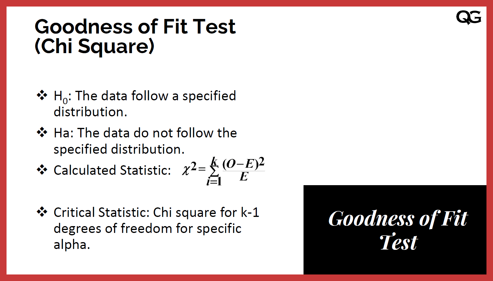
Conclusion
The Chi-Square Goodness of Fit test is a robust statistical tool used to determine how well observed data fits a hypothesized distribution. It is particularly useful for categorical data where the goal is to compare the observed frequencies with the expected frequencies under the null hypothesis.
The key steps in conducting a Chi-Square Goodness of Fit test include:
- Formulating Hypotheses: Define the null hypothesis (\(H_0\)) that the data follows a specific distribution, and the alternative hypothesis (\(H_A\)) that it does not.
- Calculating Expected Frequencies: Determine the expected frequency for each category based on the hypothesized distribution.
- Computing the Chi-Square Statistic: Use the formula \( \chi^2 = \sum \frac{(O_i - E_i)^2}{E_i} \), where \(O_i\) and \(E_i\) are the observed and expected frequencies, respectively.
- Determining the P-value: Compare the calculated Chi-Square statistic to the critical value from the Chi-Square distribution table with appropriate degrees of freedom to find the p-value.
- Making a Decision: Based on the p-value and the chosen significance level, decide whether to reject or fail to reject the null hypothesis.
Through this process, researchers can assess whether their data deviates significantly from the expected distribution, providing valuable insights into the underlying patterns and distributions in categorical data.
Overall, the Chi-Square Goodness of Fit test is essential for validating hypotheses about the distribution of categorical variables, ensuring that statistical conclusions are based on solid evidence.
Kiểm định chi bình phương của Pearson (phù hợp với mô hình) | Xác suất và Thống kê | Khan Academy
Kiểm định chi bình phương của Pearson | Khan Academy
READ MORE:
Kiểm định phù hợp của Chi-Square | Thống kê
Kiểm định phù hợp của Chi-Square


:max_bytes(150000):strip_icc()/Chi-SquareStatistic_Final_4199464-7eebcd71a4bf4d9ca1a88d278845e674.jpg)