Topic chi squared null hypothesis: The chi-squared null hypothesis is a fundamental concept in statistical analysis, used to determine if there is a significant association between categorical variables. This article delves into the chi-squared test, its applications, and how to interpret results, providing a comprehensive understanding for researchers and statisticians.
Table of Content
- Chi-Square Test and Null Hypothesis
- Introduction to Chi-Squared Tests
- Setting Up Hypotheses
- Types of Chi-Squared Tests
- Assumptions and Conditions
- Performing the Test
- Interpreting Results
- Examples of Chi-Squared Applications
- FAQs and Common Issues
- Software Tools for Chi-Squared Tests
- YOUTUBE: Tìm hiểu về kiểm định chi-square và cách áp dụng nó để kiểm tra giả thuyết null. Video này hướng dẫn chi tiết từng bước thực hiện kiểm định chi-square.
Chi-Square Test and Null Hypothesis
The chi-square (χ²) test is a statistical method used to determine if there is a significant association between two categorical variables. The test compares the observed frequencies in each category to the frequencies expected if the null hypothesis is true.
Types of Chi-Square Tests
- Chi-Square Goodness of Fit Test: This test determines if a sample data matches a population with a specific distribution. It is used with a single categorical variable.
- Chi-Square Test of Independence: This test checks if two categorical variables are independent. It is used when you have two categorical variables from a single population.
Hypotheses
For both tests, the hypotheses are structured as follows:
- Null Hypothesis (H0): Assumes no significant difference between the observed and expected frequencies.
- Alternative Hypothesis (H1): Assumes a significant difference exists between the observed and expected frequencies.
Chi-Square Test Formula
The chi-square statistic is calculated using the formula:
\[ \chi^2 = \sum \frac{(O_i - E_i)^2}{E_i} \]
where:
- \( O_i \) = observed frequency
- \( E_i \) = expected frequency
Steps to Perform a Chi-Square Test
- Set up your null and alternative hypotheses.
- Determine the expected frequencies based on the null hypothesis.
- Calculate the chi-square statistic using the formula.
- Determine the degrees of freedom and the critical value from the chi-square distribution table.
- Compare the chi-square statistic to the critical value to decide whether to reject the null hypothesis.
Example of Chi-Square Test of Independence
Consider a study examining the relationship between a city's intervention methods and household recycling behavior:
| Intervention | Recycles | Does Not Recycle | Total |
|---|---|---|---|
| Flyer | 89 | 9 | 98 |
| Phone Call | 84 | 8 | 92 |
| Control | 86 | 24 | 110 |
| Total | 259 | 41 | 300 |
To test if the intervention type affects recycling behavior, you would perform a chi-square test of independence, comparing observed and expected frequencies.
Conclusion
By comparing the chi-square statistic to the critical value, you can determine if there is a significant relationship between the variables. If the chi-square statistic exceeds the critical value, the null hypothesis is rejected, indicating a significant association.
:max_bytes(150000):strip_icc()/Chi-SquareStatistic_Final_4199464-7eebcd71a4bf4d9ca1a88d278845e674.jpg)
READ MORE:
Introduction to Chi-Squared Tests
The Chi-squared test is a statistical method used to determine if there is a significant association between two categorical variables or if an observed distribution fits an expected distribution. There are two main types of Chi-squared tests: the Chi-squared test of independence and the Chi-squared goodness of fit test.
The Chi-squared test of independence assesses whether two categorical variables are independent by comparing the observed frequencies in a contingency table to the frequencies expected if the variables were independent. On the other hand, the Chi-squared goodness of fit test evaluates how well an observed distribution of a single categorical variable matches an expected distribution based on a theoretical model.
The steps to perform a Chi-squared test typically include:
- Formulating the null and alternative hypotheses.
- Choosing a significance level (alpha).
- Calculating the expected frequencies based on the null hypothesis.
- Computing the Chi-squared statistic using the formula:
\[ \chi^2 = \sum \frac{(O_i - E_i)^2}{E_i} \] where \(O_i\) represents the observed frequency and \(E_i\) represents the expected frequency for each category. - Comparing the computed Chi-squared statistic to the critical value from the Chi-squared distribution table with the appropriate degrees of freedom.
- Drawing a conclusion based on the comparison: if the Chi-squared statistic exceeds the critical value, the null hypothesis is rejected.
Chi-squared tests are widely used in various fields such as genetics, marketing, and social sciences to test hypotheses about categorical data. They provide a robust method for evaluating the fit between observed and expected data and for identifying relationships between categorical variables.
Setting Up Hypotheses
When performing a chi-squared test, setting up hypotheses is a crucial first step. The hypotheses are statements about the population parameters that we aim to test with our sample data. There are two primary types of hypotheses involved in a chi-squared test: the null hypothesis (\(H_0\)) and the alternative hypothesis (\(H_1\)).
- Null Hypothesis (\(H_0\)): This hypothesis states that there is no significant difference between the observed and expected frequencies. It usually represents a statement of no effect or no association.
- Alternative Hypothesis (\(H_1\)): This hypothesis contradicts the null hypothesis. It states that there is a significant difference between the observed and expected frequencies, indicating an effect or association.
To illustrate, consider a chi-squared test of independence to determine if two categorical variables, such as gender and political preference, are related.
- Define the null and alternative hypotheses:
- \(H_0\): Gender and political preference are independent.
- \(H_1\): Gender and political preference are not independent.
- Decide on the significance level (\(\alpha\)), commonly set at 0.05.
- Calculate the expected frequencies for each category using the formula: \[ E = \frac{(\text{Row Total} \times \text{Column Total})}{\text{Grand Total}} \]
- Compute the chi-squared test statistic using the formula: \[ \chi^2 = \sum \frac{(O - E)^2}{E} \] where \(O\) is the observed frequency and \(E\) is the expected frequency.
- Determine the degrees of freedom, given by: \[ \text{Degrees of Freedom} = (\text{Number of Rows} - 1) \times (\text{Number of Columns} - 1)
- Compare the chi-squared statistic to the critical value from the chi-squared distribution table. If the test statistic exceeds the critical value, reject the null hypothesis.
Following these steps ensures a systematic approach to setting up and testing hypotheses using the chi-squared method.
Types of Chi-Squared Tests
The Chi-squared test is a versatile statistical method used to examine the relationships between categorical variables. There are several types of Chi-squared tests, each serving a distinct purpose in hypothesis testing.
- Chi-Square Test of Independence
- Formulate the hypotheses:
- Null hypothesis (\(H_0\)): The variables are independent.
- Alternative hypothesis (\(H_a\)): The variables are not independent.
- Calculate the expected frequencies for each cell in the contingency table.
- Compute the Chi-square statistic: \[ \chi^2 = \sum \frac{(O_i - E_i)^2}{E_i} \] where \(O_i\) is the observed frequency and \(E_i\) is the expected frequency.
- Compare the computed \(\chi^2\) value with the critical value from the Chi-square distribution table, using the appropriate degrees of freedom.
- Make a decision to reject or fail to reject the null hypothesis.
- Chi-Square Goodness of Fit Test
- Formulate the hypotheses:
- Null hypothesis (\(H_0\)): The observed frequencies match the expected frequencies.
- Alternative hypothesis (\(H_a\)): The observed frequencies do not match the expected frequencies.
- Determine the expected frequencies for each category based on the specified distribution.
- Compute the Chi-square statistic using the same formula as in the test of independence.
- Compare the \(\chi^2\) value with the critical value from the Chi-square distribution table.
- Decide whether to reject the null hypothesis.
- Chi-Square Test for Homogeneity
- Formulate the hypotheses:
- Null hypothesis (\(H_0\)): The distributions are the same across different populations.
- Alternative hypothesis (\(H_a\)): The distributions are different across populations.
- Calculate the expected frequencies for each combination of category and population.
- Compute the Chi-square statistic as before.
- Compare the \(\chi^2\) value with the critical value for the appropriate degrees of freedom.
- Make a decision on the null hypothesis.
This test determines whether two categorical variables are independent of each other. It compares the observed frequencies in a contingency table with the expected frequencies calculated under the assumption that the variables are independent.
This test checks whether the distribution of a single categorical variable matches an expected distribution. It's often used to test hypotheses about population proportions.
This test is used to determine whether different populations have the same distribution of a single categorical variable. It is similar to the test of independence but applies to multiple populations.
Each of these tests requires careful formulation of hypotheses and accurate calculation of expected frequencies to ensure valid conclusions. They are fundamental tools in statistical analysis, providing insights into the relationships between categorical variables.
Assumptions and Conditions
The Chi-Squared test is a robust statistical tool, but its validity hinges on several critical assumptions and conditions that must be met. These ensure the reliability of the test results and help avoid common pitfalls.
- Random Sampling: The data must come from a random sample of the population. Each observation should be independent, meaning the selection of one individual does not influence the selection of another.
- Expected Frequency: Each cell in the contingency table should have an expected frequency of at least 5. If more than 20% of the cells have expected frequencies below this threshold, the Chi-Squared test may not be appropriate.
- Mutual Exclusivity: Each observation must fall into one and only one category in the contingency table. This ensures that the categories are mutually exclusive and exhaustive.
- Data Type: The test is applicable to categorical data. The variables should be nominal or ordinal, and not continuous, as continuous data needs to be categorized appropriately before applying the test.
Violating these assumptions can lead to misleading results, including increased risks of Type I (false positive) or Type II (false negative) errors. Therefore, careful consideration of these conditions is crucial when planning and interpreting Chi-Squared tests.
| Assumption | Description |
| Random Sampling | Data should be collected through random sampling methods to ensure independence. |
| Expected Frequency | Each cell's expected count must be 5 or more. If not, consider combining categories or using an alternative test. |
| Mutual Exclusivity | Observations must fall into one category only, ensuring no overlap between categories. |
| Data Type | Variables must be categorical. Continuous data should be discretized appropriately. |
Adhering to these assumptions helps ensure that the Chi-Squared test produces valid and reliable results, making it a powerful tool for analyzing categorical data in various research contexts.

Performing the Test
The Chi-Squared test involves several key steps to determine if there is a significant difference between observed and expected frequencies. Follow these detailed steps:
1. Define Hypotheses
Set up your null and alternative hypotheses. The null hypothesis (H0) typically states that there is no effect or no difference, while the alternative hypothesis (H1) states that there is an effect or a difference.
- Null Hypothesis (H0): The observed frequencies do not differ from the expected frequencies.
- Alternative Hypothesis (H1): The observed frequencies differ from the expected frequencies.
2. Choose the Significance Level
Decide on the alpha (α) value, which represents the probability of rejecting the null hypothesis when it is actually true. Common choices are 0.05, 0.01, and 0.10.
3. Collect and Organize Data
Organize your data into a contingency table if you are performing a Chi-Square Test of Independence, or list observed frequencies if performing a Goodness of Fit Test.
4. Calculate Expected Frequencies
For each category or cell in the table, calculate the expected frequency using the formula:
E = \dfrac{(\text{Row Total} \times \text{Column Total})}{\text{Grand Total}}
5. Compute the Chi-Squared Statistic
Use the Chi-Squared formula to calculate the test statistic:
X^2 = \sum \dfrac{(O - E)^2}{E}
Where O is the observed frequency and E is the expected frequency.
6. Determine Degrees of Freedom
The degrees of freedom (df) depend on the type of test:
- Goodness of Fit Test: df = number of categories - 1
- Test of Independence: df = (number of rows - 1) × (number of columns - 1)
7. Find the Critical Value
Using a Chi-Square distribution table, find the critical value corresponding to your calculated degrees of freedom and chosen significance level.
8. Compare and Conclude
Compare your calculated Chi-Squared statistic to the critical value:
- If X2 is greater than the critical value, reject the null hypothesis (there is a significant difference).
- If X2 is less than or equal to the critical value, do not reject the null hypothesis (no significant difference).
Example Calculation
Suppose you are testing if a die is fair. You roll it 60 times and get the following observed frequencies for each face:
- Face 1: 10
- Face 2: 8
- Face 3: 12
- Face 4: 14
- Face 5: 9
- Face 6: 7
Expected frequency for each face (E) = 60 / 6 = 10
Calculate X2:
| Face | O | E | (O - E) | (O - E)2 | (O - E)2 / E |
|---|---|---|---|---|---|
| 1 | 10 | 10 | 0 | 0 | 0 |
| 2 | 8 | 10 | -2 | 4 | 0.4 |
| 3 | 12 | 10 | 2 | 4 | 0.4 |
| 4 | 14 | 10 | 4 | 16 | 1.6 |
| 5 | 9 | 10 | -1 | 1 | 0.1 |
| 6 | 7 | 10 | -3 | 9 | 0.9 |
X2 = 0 + 0.4 + 0.4 + 1.6 + 0.1 + 0.9 = 3.4
With df = 5 and α = 0.05, the critical value from the Chi-Square distribution table is 11.07. Since 3.4 < 11.07, we fail to reject the null hypothesis, indicating that the die appears to be fair.
Interpreting Results
After performing a chi-squared test, interpreting the results involves several key steps to understand the statistical significance and the implications of your findings. Here are the steps to effectively interpret the results:
-
Compare the P-value to the Significance Level
The p-value indicates the probability that the observed differences are due to chance. Compare the p-value to your chosen significance level (α), typically set at 0.05.
- If P-value ≤ α: Reject the null hypothesis (H0). This indicates that there is a statistically significant association between the variables.
- If P-value > α: Fail to reject the null hypothesis. This suggests that there is not enough evidence to conclude that the variables are associated.
-
Examine the Chi-Square Statistic
The chi-square statistic (χ2) is calculated by summing the squared differences between observed and expected frequencies, divided by the expected frequencies. Larger values of χ2 indicate greater discrepancies between observed and expected data.
-
Assess the Degrees of Freedom (DF)
The degrees of freedom for a chi-squared test are determined by the number of categories minus one. The DF helps to determine the critical value of χ2 for a given significance level.
-
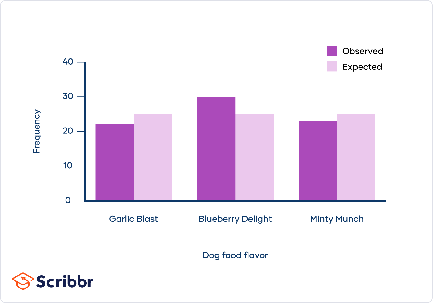
Compare Observed and Expected Frequencies
Analyze the observed frequencies (actual data) against the expected frequencies (what you would expect if the null hypothesis were true). Large deviations suggest a significant difference.
Category Observed Frequency Expected Frequency Contribution to χ2 Category 1 48 56.08 1.1637 Category 2 76 60.78 3.8088 Category 3 36 43.14 1.1809 -
Identify Key Contributors
Look for the cells or categories that contribute the most to the chi-square statistic. These are the areas where the observed data deviates most from what was expected and could indicate areas of interest or concern.
By following these steps, you can determine whether your data provides sufficient evidence to support rejecting the null hypothesis, thereby suggesting an association between the variables under study.
Examples of Chi-Squared Applications
Chi-squared tests are widely used in various fields to determine whether there is a significant association between categorical variables. Here are some detailed examples:
-
Example 1: Goodness of Fit
Suppose a geneticist wants to test a hypothesis about the distribution of blood types in a population. According to genetic theory, the proportions of blood types A, B, AB, and O are 25%, 25%, 25%, and 25%, respectively. The observed counts in a sample of 400 individuals are:
Blood Type Observed Count Expected Count A 110 100 B 90 100 AB 95 100 O 105 100 To test the goodness of fit, we calculate the chi-squared statistic:
\[
\chi^2 = \sum \frac{(O_i - E_i)^2}{E_i} = \frac{(110 - 100)^2}{100} + \frac{(90 - 100)^2}{100} + \frac{(95 - 100)^2}{100} + \frac{(105 - 100)^2}{100} = 2.5
\]With a significance level of 0.05 and 3 degrees of freedom, we compare the chi-squared statistic to the critical value from the chi-squared distribution table. If the calculated value is less than the critical value, we fail to reject the null hypothesis, indicating a good fit.
-
Example 2: Test of Independence
Consider a study to determine if there is an association between gender and political party preference. A random sample of 500 voters is surveyed with the following results:
Gender Republican Democrat Independent Total Male 120 90 40 250 Female 110 95 45 250 Total 230 185 85 500 The hypotheses for the chi-squared test of independence are:
- \(H_0\): Gender and political party preference are independent.
- \(H_1\): Gender and political party preference are not independent.
We calculate the expected counts for each cell using the formula:
\[
E_{ij} = \frac{(\text{row total}) \times (\text{column total})}{\text{grand total}}
\]For example, the expected count for male Republicans is:
\[
E = \frac{250 \times 230}{500} = 115
\]We then compute the chi-squared statistic:
\[
\chi^2 = \sum \frac{(O_i - E_i)^2}{E_i}
\]After calculating the test statistic and comparing it to the critical value with appropriate degrees of freedom, we determine whether to reject the null hypothesis. If the p-value is less than the significance level (e.g., 0.05), we reject the null hypothesis, indicating a significant association between gender and political party preference.
FAQs and Common Issues
Here we address some frequently asked questions and common issues encountered with chi-squared tests:
FAQs
-
What is the null hypothesis in a chi-squared test?
The null hypothesis (\(H_0\)) in a chi-squared test states that there is no significant difference between the observed and expected frequencies. It posits that any observed deviations are due to random chance.
-
How do I interpret the p-value in a chi-squared test?
The p-value indicates the probability of obtaining a chi-squared statistic at least as extreme as the one calculated from your data, assuming the null hypothesis is true. A low p-value (typically < 0.05) suggests that the observed deviation is unlikely to have occurred by chance, leading to the rejection of the null hypothesis.
-
What are the assumptions of the chi-squared test?
- Independence: Observations must be independent of each other.
- Sample Size: All expected frequencies should be at least 1, and no more than 20% of expected frequencies should be less than 5.
- Data Level: The variables should be categorical.
-
How do I calculate the degrees of freedom for a chi-squared test?
The degrees of freedom (df) for a chi-squared test are calculated based on the number of categories. For a goodness-of-fit test, df is the number of categories minus one (df = n - 1). For a test of independence, df is calculated as (rows - 1) * (columns - 1).
Common Issues
-
Small Expected Frequencies
If expected frequencies are too low, the chi-squared test might not be valid. To address this, combine categories or use a different statistical test, such as Fisher's exact test, which is more suitable for small sample sizes.
-
Non-Independent Observations
Independence of observations is crucial for the validity of the chi-squared test. Ensure your data collection methods do not introduce dependencies between observations.
-
Incorrectly Categorized Data
Ensure that data is correctly categorized and that categories are mutually exclusive and collectively exhaustive. Misclassification can lead to incorrect conclusions.
-
Misinterpretation of Results
Remember that a significant chi-squared result does not imply causation but rather an association between variables. Carefully consider other possible explanations and confounding factors before drawing conclusions.
Software Tools for Chi-Squared Tests
Several software tools are available to perform Chi-Squared tests efficiently. These tools provide user-friendly interfaces and robust statistical analysis capabilities. Below are some of the popular software tools:
- JASP
JASP is a free and user-friendly statistical software that provides a range of tests, including the Chi-Square test. It allows users to easily perform both Chi-Square Goodness of Fit and Chi-Square Test of Independence. Users can input data and specify the null hypothesis directly in the software, which then calculates the Chi-Square statistic and provides a comprehensive results table. JASP also offers visualization tools to help interpret the results.
- SPSS
SPSS (Statistical Package for the Social Sciences) is a widely used program for statistical analysis in social science. It includes a dedicated module for performing Chi-Squared tests. Users can enter their data into a spreadsheet interface, specify the type of Chi-Squared test they wish to conduct, and receive detailed outputs including Chi-Square values, degrees of freedom, and p-values. SPSS also provides graphical representations of the data and test results.
- Minitab
Minitab is another popular statistical software that supports Chi-Squared tests. It simplifies the process of conducting these tests by offering step-by-step guidance through its user interface. Users can easily input their categorical data, and Minitab will compute the expected frequencies, Chi-Square statistic, and associated p-values. Additionally, Minitab provides tools for visual data analysis, which helps in understanding the results better.
- R
R is a programming language and free software environment for statistical computing. It provides extensive support for Chi-Squared tests through various packages such as
statsandMASS. Users can write scripts to perform Chi-Squared tests, allowing for highly customizable and reproducible analysis. R also supports advanced data visualization techniques to interpret the test results effectively.
Each of these tools has its strengths, and the choice of software may depend on the user's familiarity with the tool, the complexity of the data, and the specific requirements of the analysis. These tools not only facilitate the calculation of Chi-Square statistics but also help in the interpretation and visualization of the results, making them invaluable for statistical analysis in various fields.
Tìm hiểu về kiểm định chi-square và cách áp dụng nó để kiểm tra giả thuyết null. Video này hướng dẫn chi tiết từng bước thực hiện kiểm định chi-square.
Kiểm Định Chi-Square
READ MORE:
Khám phá thống kê chi-square và cách sử dụng nó trong kiểm định giả thuyết. Video này từ Khan Academy cung cấp hướng dẫn chi tiết và dễ hiểu về chủ đề này.
Thống kê Chi-Square cho kiểm định giả thuyết | AP Statistics | Khan Academy