Topic chi square null hypothesis example: Explore the chi-square null hypothesis through detailed examples in this comprehensive guide. Learn how to formulate hypotheses, calculate expected frequencies, and interpret chi-square test results. Perfect for students, researchers, and anyone interested in statistical methods, this article will enhance your understanding of chi-square tests and their applications.
Table of Content
- Chi-Square Test: Null Hypothesis Example
- Introduction to Chi-Square Test
- Formulating Null and Alternative Hypotheses
- Types of Chi-Square Tests
- Chi-Square Test for Independence
- Chi-Square Goodness of Fit Test
- Calculating Expected Frequencies
- Chi-Square Test Statistic Formula
- Degrees of Freedom in Chi-Square Test
- Using Chi-Square Distribution Table
- Interpreting Chi-Square Results
- Example of Chi-Square Test for Independence
- Example of Chi-Square Goodness of Fit Test
- Common Applications of Chi-Square Tests
- Assumptions and Limitations of Chi-Square Test
- YOUTUBE: Video về Kiểm Định Chi-Square giới thiệu cách sử dụng kiểm định này trong thống kê, phù hợp với ví dụ giả thuyết không chi-square.
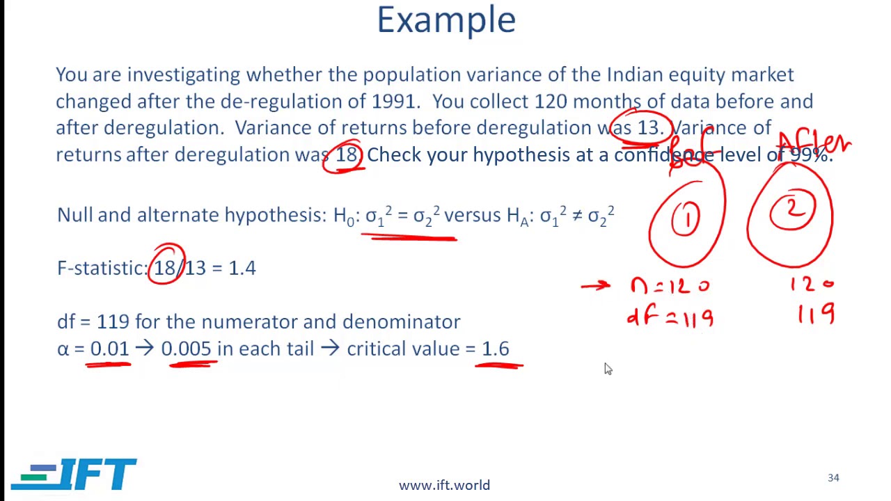
Chi-Square Test: Null Hypothesis Example
The chi-square test is a statistical method used to determine if there is a significant association between categorical variables. This test compares the observed frequencies of events to the expected frequencies under the null hypothesis. Below is an example illustrating the chi-square test and the formulation of the null hypothesis.
Example: Testing the Independence of Two Variables
Suppose we want to test whether there is a relationship between gender (male or female) and preference for a new product (like or dislike). We collect data from a sample of 100 individuals, resulting in the following contingency table:
| Like | Dislike | Total | |
| Male | 30 | 20 | 50 |
| Female | 10 | 40 | 50 |
| Total | 40 | 60 | 100 |
Null Hypothesis (\(H_0\))
The null hypothesis states that there is no association between gender and product preference. In other words, gender and preference are independent.
\[ H_0: \text{Gender and product preference are independent} \]
Alternative Hypothesis (\(H_1\))
The alternative hypothesis states that there is an association between gender and product preference. In other words, gender and preference are not independent.
\[ H_1: \text{Gender and product preference are not independent} \]
Expected Frequencies
The expected frequency for each cell under the null hypothesis can be calculated using the formula:
\[ E_{ij} = \frac{(Row\ Total\ for\ i)(Column\ Total\ for\ j)}{Grand\ Total} \]
Using this formula, we calculate the expected frequencies:
- Expected frequency for Male and Like: \[ E_{11} = \frac{50 \times 40}{100} = 20 \]
- Expected frequency for Male and Dislike: \[ E_{12} = \frac{50 \times 60}{100} = 30 \]
- Expected frequency for Female and Like: \[ E_{21} = \frac{50 \times 40}{100} = 20 \]
- Expected frequency for Female and Dislike: \[ E_{22} = \frac{50 \times 60}{100} = 30 \]
Chi-Square Statistic
The chi-square statistic is calculated using the formula:
\[ \chi^2 = \sum \frac{(O_{ij} - E_{ij})^2}{E_{ij}} \]
Where \(O_{ij}\) is the observed frequency and \(E_{ij}\) is the expected frequency. Substituting the values, we get:
\[ \chi^2 = \frac{(30 - 20)^2}{20} + \frac{(20 - 30)^2}{30} + \frac{(10 - 20)^2}{20} + \frac{(40 - 30)^2}{30} \]
\[ \chi^2 = \frac{100}{20} + \frac{100}{30} + \frac{100}{20} + \frac{100}{30} \]
\[ \chi^2 = 5 + \frac{10}{3} + 5 + \frac{10}{3} \]
\[ \chi^2 \approx 13.33 \]
Conclusion
We compare the calculated chi-square statistic to the critical value from the chi-square distribution table with the appropriate degrees of freedom (df). For a 2x2 table, df = (2-1)(2-1) = 1. If the calculated chi-square value exceeds the critical value, we reject the null hypothesis, suggesting that there is a significant association between gender and product preference.
READ MORE:
Introduction to Chi-Square Test
The chi-square test is a statistical method used to determine if there is a significant association between categorical variables. It helps in testing hypotheses about the distribution of categorical data. There are two main types of chi-square tests: the Chi-Square Test for Independence and the Chi-Square Goodness of Fit Test.
Here’s a step-by-step introduction to understanding and performing a chi-square test:
-
Formulate Hypotheses:
- Null Hypothesis (\(H_0\)): Assumes that there is no significant association between the variables.
- Alternative Hypothesis (\(H_1\)): Assumes that there is a significant association between the variables.
-
Construct a Contingency Table:
Create a table to display the frequency distribution of the variables. For example, consider a survey that records preferences for a new product among males and females.
Like Dislike Total Male 30 20 50 Female 10 40 50 Total 40 60 100 -
Calculate Expected Frequencies:
The expected frequency for each cell in the table is calculated using the formula:
\[ E_{ij} = \frac{(Row\ Total\ for\ i)(Column\ Total\ for\ j)}{Grand\ Total} \]
- Expected frequency for Male and Like: \[ E_{11} = \frac{50 \times 40}{100} = 20 \]
- Expected frequency for Male and Dislike: \[ E_{12} = \frac{50 \times 60}{100} = 30 \]
- Expected frequency for Female and Like: \[ E_{21} = \frac{50 \times 40}{100} = 20 \]
- Expected frequency for Female and Dislike: \[ E_{22} = \frac{50 \times 60}{100} = 30 \]
-
Calculate the Chi-Square Statistic:
The chi-square statistic is calculated using the formula:
\[ \chi^2 = \sum \frac{(O_{ij} - E_{ij})^2}{E_{ij}} \]
Where \(O_{ij}\) is the observed frequency and \(E_{ij}\) is the expected frequency. Using the values from the example:
\[ \chi^2 = \frac{(30 - 20)^2}{20} + \frac{(20 - 30)^2}{30} + \frac{(10 - 20)^2}{20} + \frac{(40 - 30)^2}{30} \]
\[ \chi^2 = \frac{100}{20} + \frac{100}{30} + \frac{100}{20} + \frac{100}{30} \]
\[ \chi^2 = 5 + \frac{10}{3} + 5 + \frac{10}{3} \]
\[ \chi^2 \approx 13.33 \]
-
Determine the Degrees of Freedom:
Degrees of freedom for a chi-square test are calculated as:
\[ df = (Number\ of\ Rows - 1) \times (Number\ of\ Columns - 1) \]
For a 2x2 table, \( df = (2-1)(2-1) = 1 \).
-
Compare to the Critical Value:
Using the chi-square distribution table, compare the calculated chi-square statistic with the critical value at the desired significance level (e.g., 0.05). If the chi-square statistic exceeds the critical value, reject the null hypothesis.
Formulating Null and Alternative Hypotheses
Formulating clear and precise hypotheses is a critical step in the chi-square test process. These hypotheses will guide your analysis and interpretation of the data. Here's a detailed step-by-step guide to formulating null and alternative hypotheses for a chi-square test:
-
Understand the Research Question:
Before formulating the hypotheses, clearly define the research question. For example, you may want to know if there is an association between gender and product preference.
-
Identify the Variables:
Determine the categorical variables involved. In our example, the variables are gender (male, female) and product preference (like, dislike).
-
Formulate the Null Hypothesis (\(H_0\)):
The null hypothesis states that there is no association between the variables. It assumes that any observed differences are due to random chance.
\[ H_0: \text{Gender and product preference are independent} \]
-
Formulate the Alternative Hypothesis (\(H_1\)):
The alternative hypothesis states that there is an association between the variables. It suggests that the observed differences are not due to random chance but to a specific relationship.
\[ H_1: \text{Gender and product preference are not independent} \]
-
Express Hypotheses in Terms of Expected Frequencies:
When formulating these hypotheses, consider the expected frequencies if the null hypothesis is true. For example, the expected number of males and females liking or disliking the product should match the overall proportions if there is no association.
-
State Hypotheses Clearly and Concisely:
Ensure that both hypotheses are stated clearly and concisely. This clarity will help in accurately interpreting the results of the chi-square test.
By carefully formulating the null and alternative hypotheses, you set the foundation for a rigorous chi-square test that can provide meaningful insights into your data. In our example:
- Null Hypothesis (\(H_0\)): Gender and product preference are independent.
- Alternative Hypothesis (\(H_1\)): Gender and product preference are not independent.
These hypotheses will then be tested using the chi-square statistic to determine if the observed data significantly deviates from the expected distribution under the null hypothesis.
Types of Chi-Square Tests
The chi-square test is a versatile statistical tool used to analyze categorical data. There are two main types of chi-square tests: the Chi-Square Test for Independence and the Chi-Square Goodness of Fit Test. Each test serves a distinct purpose and is used in different scenarios. Below is a detailed overview of these types of chi-square tests:
-
Chi-Square Test for Independence:
This test is used to determine if there is a significant association between two categorical variables. It assesses whether the distribution of one variable is independent of the other. For example, it can be used to test if gender is related to product preference.
-
Example:
Consider a survey of 100 individuals categorized by gender (male, female) and their preference for a new product (like, dislike). The observed frequencies are arranged in a contingency table.
Like Dislike Total Male 30 20 50 Female 10 40 50 Total 40 60 100 The null hypothesis (\(H_0\)) states that gender and product preference are independent. The chi-square test for independence is used to evaluate this hypothesis.
-
Example:
-
Chi-Square Goodness of Fit Test:
This test is used to determine if the observed frequency distribution of a single categorical variable matches an expected distribution. It assesses how well the observed data fit a theoretical distribution.
-
Example:
Suppose a dice is rolled 60 times, and the observed frequencies of each outcome (1 through 6) are recorded. We want to test if the dice is fair, meaning each outcome is equally likely with an expected frequency of 10 for each face.
Outcome Observed Frequency Expected Frequency 1 8 10 2 12 10 3 9 10 4 11 10 5 10 10 6 10 10 The null hypothesis (\(H_0\)) states that the dice is fair, meaning the observed frequencies follow a uniform distribution. The chi-square goodness of fit test evaluates this hypothesis.
-
Example:
By understanding the different types of chi-square tests, researchers can select the appropriate test based on their specific research questions and data. Both tests play a crucial role in analyzing categorical data and drawing meaningful conclusions.
Chi-Square Test for Independence
The Chi-Square Test for Independence is used to determine whether there is a significant association between two categorical variables. This test helps to understand if the distribution of one variable is independent of the distribution of another variable. Here’s a step-by-step guide to performing a Chi-Square Test for Independence:
-
Formulate the Hypotheses:
- Null Hypothesis (\(H_0\)): Assumes that there is no association between the two variables (they are independent).
- Alternative Hypothesis (\(H_1\)): Assumes that there is an association between the two variables (they are not independent).
-
Collect and Organize Data:
Collect the data and organize it into a contingency table. For example, consider a survey of 100 individuals to determine if gender influences product preference:
Like Dislike Total Male 30 20 50 Female 10 40 50 Total 40 60 100 -
Calculate the Expected Frequencies:
Expected frequencies are calculated under the assumption that the null hypothesis is true, using the formula:
\[ E_{ij} = \frac{(Row\ Total\ for\ i)(Column\ Total\ for\ j)}{Grand\ Total} \]
- Expected frequency for Male and Like: \[ E_{11} = \frac{50 \times 40}{100} = 20 \]
- Expected frequency for Male and Dislike: \[ E_{12} = \frac{50 \times 60}{100} = 30 \]
- Expected frequency for Female and Like: \[ E_{21} = \frac{50 \times 40}{100} = 20 \]
- Expected frequency for Female and Dislike: \[ E_{22} = \frac{50 \times 60}{100} = 30 \]
-
Compute the Chi-Square Statistic:
The chi-square statistic is computed using the formula:
\[ \chi^2 = \sum \frac{(O_{ij} - E_{ij})^2}{E_{ij}} \]
Where \(O_{ij}\) is the observed frequency and \(E_{ij}\) is the expected frequency. Substituting the values:
\[ \chi^2 = \frac{(30 - 20)^2}{20} + \frac{(20 - 30)^2}{30} + \frac{(10 - 20)^2}{20} + \frac{(40 - 30)^2}{30} \]
\[ \chi^2 = \frac{100}{20} + \frac{100}{30} + \frac{100}{20} + \frac{100}{30} \]
\[ \chi^2 = 5 + \frac{10}{3} + 5 + \frac{10}{3} \]
\[ \chi^2 \approx 13.33 \]
-
Determine the Degrees of Freedom:
Degrees of freedom for a chi-square test for independence are calculated as:
\[ df = (Number\ of\ Rows - 1) \times (Number\ of\ Columns - 1) \]
For a 2x2 table, \( df = (2-1)(2-1) = 1 \).
-
Compare to the Critical Value:
Using the chi-square distribution table, compare the calculated chi-square statistic with the critical value at the desired significance level (e.g., 0.05). If the chi-square statistic exceeds the critical value, reject the null hypothesis.
The Chi-Square Test for Independence helps determine whether there is a significant relationship between two categorical variables. By following these steps, researchers can effectively test their hypotheses and draw meaningful conclusions from their data.

Chi-Square Goodness of Fit Test
The Chi-Square Goodness of Fit Test is used to determine whether the observed frequency distribution of a categorical variable matches an expected distribution. This test helps assess how well the observed data fit a theoretical model. Here’s a detailed, step-by-step guide to performing a Chi-Square Goodness of Fit Test:
-
Formulate the Hypotheses:
- Null Hypothesis (\(H_0\)): Assumes that the observed frequency distribution matches the expected distribution.
- Alternative Hypothesis (\(H_1\)): Assumes that the observed frequency distribution does not match the expected distribution.
-
Collect and Organize Data:
Collect the observed data and define the expected frequencies based on a theoretical distribution. For example, suppose we roll a die 60 times to test if it is fair:
Outcome Observed Frequency Expected Frequency 1 8 10 2 12 10 3 9 10 4 11 10 5 10 10 6 10 10 -
Calculate the Expected Frequencies:
For a fair die, the expected frequency for each outcome is calculated by:
\[ E_i = \frac{Total\ number\ of\ trials}{Number\ of\ outcomes} \]
For our example, with 60 rolls and 6 possible outcomes, the expected frequency for each outcome is:
\[ E_i = \frac{60}{6} = 10 \]
-
Compute the Chi-Square Statistic:
The chi-square statistic is computed using the formula:
\[ \chi^2 = \sum \frac{(O_i - E_i)^2}{E_i} \]
Where \(O_i\) is the observed frequency and \(E_i\) is the expected frequency. Substituting the values from our example:
\[ \chi^2 = \frac{(8 - 10)^2}{10} + \frac{(12 - 10)^2}{10} + \frac{(9 - 10)^2}{10} + \frac{(11 - 10)^2}{10} + \frac{(10 - 10)^2}{10} + \frac{(10 - 10)^2}{10} \]
\[ \chi^2 = \frac{4}{10} + \frac{4}{10} + \frac{1}{10} + \frac{1}{10} + \frac{0}{10} + \frac{0}{10} \]
\[ \chi^2 = 0.4 + 0.4 + 0.1 + 0.1 + 0 + 0 \]
\[ \chi^2 = 1 \]
-
Determine the Degrees of Freedom:
Degrees of freedom for a chi-square goodness of fit test are calculated as:
\[ df = Number\ of\ categories - 1 \]
For our example with 6 outcomes, \( df = 6 - 1 = 5 \).
-
Compare to the Critical Value:
Using the chi-square distribution table, compare the calculated chi-square statistic with the critical value at the desired significance level (e.g., 0.05). If the chi-square statistic is less than the critical value, fail to reject the null hypothesis.
The Chi-Square Goodness of Fit Test helps determine whether an observed frequency distribution differs from a theoretical distribution. By following these steps, researchers can test hypotheses about the distribution of categorical data and draw meaningful conclusions.
Calculating Expected Frequencies
Calculating expected frequencies is a crucial step in conducting a chi-square test. The expected frequencies represent the counts we would expect in each category if the null hypothesis were true. Here’s a detailed, step-by-step guide on how to calculate expected frequencies:
-
Identify the Observed Frequencies:
First, organize your observed data into a contingency table. For example, consider a study on the relationship between gender and product preference:
Like Dislike Total Male 30 20 50 Female 10 40 50 Total 40 60 100 -
Calculate the Expected Frequencies:
Expected frequencies (\(E_{ij}\)) are calculated using the formula:
\[ E_{ij} = \frac{(Row\ Total\ for\ i)(Column\ Total\ for\ j)}{Grand\ Total} \]
Apply this formula to each cell in the table:
- Expected frequency for Male and Like: \[ E_{11} = \frac{50 \times 40}{100} = 20 \]
- Expected frequency for Male and Dislike: \[ E_{12} = \frac{50 \times 60}{100} = 30 \]
- Expected frequency for Female and Like: \[ E_{21} = \frac{50 \times 40}{100} = 20 \]
- Expected frequency for Female and Dislike: \[ E_{22} = \frac{50 \times 60}{100} = 30 \]
-
Create the Expected Frequencies Table:
Construct a table to display the expected frequencies calculated in the previous step:
Like Dislike Total Male 20 30 50 Female 20 30 50 Total 40 60 100 -
Compare Observed and Expected Frequencies:
With the observed and expected frequencies organized, you are now ready to perform the chi-square test. The next steps will involve calculating the chi-square statistic and comparing it to the critical value to determine if there is a significant association between the variables.
By following these steps, researchers can accurately calculate the expected frequencies needed to conduct a chi-square test. This process ensures that the test is based on a sound statistical foundation, allowing for meaningful and reliable conclusions.
Chi-Square Test Statistic Formula
The Chi-Square test statistic is a measure used in statistical tests to determine whether there is a significant difference between the observed and expected frequencies in categorical data. Here’s a detailed, step-by-step guide to understanding and calculating the Chi-Square test statistic:
-
Understanding the Formula:
The formula for the Chi-Square test statistic is:
\[ \chi^2 = \sum \frac{(O_i - E_i)^2}{E_i} \]
Where:
- \( \chi^2 \) = Chi-Square test statistic
- \( O_i \) = Observed frequency for category \(i\)
- \( E_i \) = Expected frequency for category \(i\)
-
Identify Observed Frequencies:
Collect the observed frequencies for each category and organize them into a contingency table. For example, consider a survey on the relationship between education level and job satisfaction:
Satisfied Neutral Dissatisfied Total High School 50 30 20 100 Bachelor's 30 40 30 100 Master's 20 30 50 100 Total 100 100 100 300 -
Calculate Expected Frequencies:
Use the formula for expected frequencies:
\[ E_{ij} = \frac{(Row\ Total_i \times Column\ Total_j)}{Grand\ Total} \]
For example, the expected frequency for "High School and Satisfied" is:
\[ E_{11} = \frac{100 \times 100}{300} = \frac{10000}{300} \approx 33.33 \]
-
Compute the Chi-Square Statistic:
Calculate the chi-square statistic using the observed and expected frequencies. For each cell, compute:
\[ \chi^2 = \sum \frac{(O_i - E_i)^2}{E_i} \]
- For "High School and Satisfied": \[ \frac{(50 - 33.33)^2}{33.33} \approx 8.33 \]
- For "High School and Neutral": \[ \frac{(30 - 33.33)^2}{33.33} \approx 0.33 \]
- For "High School and Dissatisfied": \[ \frac{(20 - 33.33)^2}{33.33} \approx 5.33 \]
Sum all these values to get the chi-square statistic:
\[ \chi^2 = 8.33 + 0.33 + 5.33 + \ldots \]
-
Compare to the Critical Value:
Determine the degrees of freedom for the test:
\[ df = (Number\ of\ Rows - 1) \times (Number\ of\ Columns - 1) \]
For our example, \( df = (3 - 1)(3 - 1) = 4 \).
Using a chi-square distribution table, compare the calculated chi-square statistic to the critical value at the desired significance level (e.g., 0.05). If the chi-square statistic is greater than the critical value, reject the null hypothesis.
By following these steps, researchers can accurately calculate the chi-square test statistic and determine whether there is a significant difference between the observed and expected frequencies in their data.
Degrees of Freedom in Chi-Square Test
The concept of degrees of freedom is critical in performing a Chi-Square test. Degrees of freedom (df) refer to the number of independent values or quantities that can be assigned to a statistical distribution. In the context of the Chi-Square test, degrees of freedom help determine the critical value from the Chi-Square distribution table.
There are different ways to calculate degrees of freedom depending on the type of Chi-Square test being performed. Here are the formulas for the most common types:
Degrees of Freedom for Chi-Square Test for Independence
When performing a Chi-Square test for independence, the degrees of freedom are calculated using the formula:
\[ df = (r - 1) \times (c - 1) \]
where \( r \) is the number of rows and \( c \) is the number of columns in the contingency table. This formula accounts for the fact that once certain values are fixed, the rest are determined by the marginal totals.
For example, if you have a 3x3 table:
- Number of rows, \( r = 3 \)
- Number of columns, \( c = 3 \)
- Degrees of freedom, \( df = (3 - 1) \times (3 - 1) = 2 \times 2 = 4 \)
Degrees of Freedom for Chi-Square Goodness of Fit Test
For the Chi-Square Goodness of Fit test, the degrees of freedom are calculated using the formula:
\[ df = n - 1 \]
where \( n \) is the number of categories or groups. This formula accounts for the fact that the observed frequencies must sum to the total sample size, leaving one less degree of freedom.
For example, if you have 5 categories:
- Number of categories, \( n = 5 \)
- Degrees of freedom, \( df = 5 - 1 = 4 \)
Importance of Degrees of Freedom
Degrees of freedom are important because they directly affect the critical value needed to determine whether to reject the null hypothesis. Higher degrees of freedom result in a larger critical value, making it harder to achieve a statistically significant result. This is because with more degrees of freedom, the distribution of the test statistic becomes broader.
Using Degrees of Freedom in Practice
To use degrees of freedom in practice:
- Calculate the degrees of freedom using the appropriate formula.
- Refer to the Chi-Square distribution table to find the critical value corresponding to the calculated degrees of freedom and the chosen significance level (e.g., 0.05).
- Compare the calculated Chi-Square test statistic to the critical value to decide whether to reject the null hypothesis.
Understanding and correctly calculating degrees of freedom is essential for the proper application of the Chi-Square test, ensuring accurate interpretation of the results.

Using Chi-Square Distribution Table
The Chi-Square distribution table is a critical tool for determining whether to reject the null hypothesis in a Chi-Square test. It provides the critical values of the Chi-Square distribution for various degrees of freedom and significance levels. Here is a step-by-step guide on how to use the Chi-Square distribution table effectively:
-
Calculate the Chi-Square Test Statistic: Compute the Chi-Square test statistic using the appropriate formula for your test (e.g., Chi-Square test for independence or Chi-Square goodness of fit test).
-
Determine the Degrees of Freedom: Calculate the degrees of freedom (df) based on the type of test being performed. For example:
- Chi-Square Test for Independence: \( df = (r - 1) \times (c - 1) \)
- Chi-Square Goodness of Fit Test: \( df = n - 1 \)
-
Select the Significance Level: Choose the significance level (\( \alpha \)) for your test, commonly set at 0.05 (5%) or 0.01 (1%). This represents the probability of rejecting the null hypothesis when it is actually true.
-
Find the Critical Value: Use the Chi-Square distribution table to find the critical value that corresponds to the calculated degrees of freedom and the chosen significance level.
Degrees of Freedom (df) 0.10 0.05 0.01 1 2.71 3.84 6.63 2 4.61 5.99 9.21 3 6.25 7.81 11.34 -
Compare the Test Statistic to the Critical Value: Compare the calculated Chi-Square test statistic to the critical value obtained from the table.
- If the test statistic is greater than the critical value, reject the null hypothesis.
- If the test statistic is less than or equal to the critical value, do not reject the null hypothesis.
Let's consider an example:
- Calculated Test Statistic: 10.2
- Degrees of Freedom: 4
- Significance Level: 0.05
- Critical Value from Table: 9.49
- Decision: Since 10.2 > 9.49, we reject the null hypothesis.
Using the Chi-Square distribution table allows you to make informed decisions about the null hypothesis based on your test results. Understanding how to navigate and interpret this table is essential for accurate statistical analysis.
Interpreting Chi-Square Results
Interpreting the results of a Chi-Square test involves understanding the test statistic, degrees of freedom, and the p-value to make informed decisions about the null hypothesis. Follow these detailed steps to interpret Chi-Square results effectively:
-
Calculate the Chi-Square Test Statistic: Ensure you have accurately calculated the Chi-Square test statistic using the relevant formula for your specific test.
-
Determine the Degrees of Freedom: Calculate the degrees of freedom (df) based on your test type:
- Chi-Square Test for Independence: \( df = (r - 1) \times (c - 1) \)
- Chi-Square Goodness of Fit Test: \( df = n - 1 \)
-
Find the Critical Value: Use the Chi-Square distribution table to find the critical value corresponding to your degrees of freedom and chosen significance level (e.g., 0.05).
-
Compare the Test Statistic to the Critical Value: Compare the calculated Chi-Square test statistic to the critical value from the Chi-Square distribution table:
- If the test statistic is greater than the critical value, reject the null hypothesis.
- If the test statistic is less than or equal to the critical value, do not reject the null hypothesis.
-
Determine the P-Value: The p-value indicates the probability of observing a test statistic as extreme as, or more extreme than, the observed value under the null hypothesis. Use statistical software or a Chi-Square distribution table to find the p-value:
- If the p-value is less than or equal to the significance level (e.g., 0.05), reject the null hypothesis.
- If the p-value is greater than the significance level, do not reject the null hypothesis.
Here is an example to illustrate the process:
- Observed Chi-Square Test Statistic: 10.2
- Degrees of Freedom: 4
- Significance Level: 0.05
- Critical Value from Table: 9.49
- Calculated P-Value: 0.037
- Decision: Since 10.2 > 9.49 and the p-value (0.037) is less than 0.05, we reject the null hypothesis.
Conclusion: The rejection of the null hypothesis suggests that there is a significant association between the variables in the Chi-Square test for independence, or that the observed frequencies significantly differ from the expected frequencies in the Chi-Square goodness of fit test.
Understanding and accurately interpreting the Chi-Square results is crucial for drawing valid conclusions from your statistical analysis. Always ensure to cross-check your calculations and refer to the Chi-Square distribution table correctly to make informed decisions.
Example of Chi-Square Test for Independence
A Chi-Square test for independence is used to determine whether there is a significant association between two categorical variables. Here is a detailed example of how to perform and interpret a Chi-Square test for independence:
Step-by-Step Example:
-
Formulate the Hypotheses:
- Null Hypothesis (H0): There is no association between the two categorical variables.
- Alternative Hypothesis (H1): There is an association between the two categorical variables.
-
Collect the Data: Suppose we have the following observed data on gender and preference for a new product:
Preference Male Female Total Like 20 30 50 Dislike 10 40 50 Total 30 70 100 -
Calculate the Expected Frequencies: The expected frequency for each cell is calculated using the formula:
\[
E = \frac{(row\ total \times column\ total)}{grand\ total}
\]For example, the expected frequency for males who like the product is:
\[
E = \frac{(50 \times 30)}{100} = 15
\]The expected frequencies table is:
Preference Male Female Total Like 15 35 50 Dislike 15 35 50 Total 30 70 100 -
Calculate the Chi-Square Test Statistic: Use the formula:
\[
\chi^2 = \sum \frac{(O - E)^2}{E}
\]For example, for males who like the product:
\[
\frac{(20 - 15)^2}{15} = \frac{25}{15} = 1.67
\]Repeat this calculation for each cell and sum the results:
Preference Male Female Like 1.67 0.71 Dislike 1.67 0.71 Total \(\chi^2\) = 1.67 + 0.71 + 1.67 + 0.71 = 4.76
-
Determine the Degrees of Freedom: The degrees of freedom (df) for the test is calculated as:
\[
df = (r - 1) \times (c - 1)
\]In this example:
\[
df = (2 - 1) \times (2 - 1) = 1
\] -
Find the Critical Value and Compare: At a significance level of 0.05 and df = 1, the critical value from the Chi-Square distribution table is 3.84.
- Since 4.76 > 3.84, we reject the null hypothesis.
-
Conclusion: There is sufficient evidence to suggest an association between gender and preference for the new product.
Example of Chi-Square Goodness of Fit Test
A Chi-Square Goodness of Fit test is used to determine whether the observed frequency distribution of a categorical variable matches an expected distribution. Here is a detailed example of how to perform and interpret a Chi-Square Goodness of Fit test:
Step-by-Step Example:
-
Formulate the Hypotheses:
- Null Hypothesis (H0): The observed frequencies match the expected frequencies.
- Alternative Hypothesis (H1): The observed frequencies do not match the expected frequencies.
-
Collect the Data: Suppose we have the following observed data on the number of customers visiting a store on different days of the week:
Day Observed Frequency Monday 50 Tuesday 30 Wednesday 20 Thursday 40 Friday 60 Total 200 -
Determine the Expected Frequencies: Suppose the store expects an equal number of customers each day. The expected frequency for each day is:
\[
E = \frac{Total\ Customers}{Number\ of\ Days} = \frac{200}{5} = 40
\]The expected frequencies table is:
Day Expected Frequency Monday 40 Tuesday 40 Wednesday 40 Thursday 40 Friday 40 -
Calculate the Chi-Square Test Statistic: Use the formula:
\[
\chi^2 = \sum \frac{(O - E)^2}{E}
\]For example, for Monday:
\[
\frac{(50 - 40)^2}{40} = \frac{100}{40} = 2.5
\]Repeat this calculation for each day and sum the results:
Day Chi-Square Contribution Monday 2.5 Tuesday 2.5 Wednesday 10 Thursday 0 Friday 10 Total 25 Total \(\chi^2\) = 2.5 + 2.5 + 10 + 0 + 10 = 25
-
Determine the Degrees of Freedom: The degrees of freedom (df) for the test is calculated as:
\[
df = n - 1
\]In this example:
\[
df = 5 - 1 = 4
\] -
Find the Critical Value and Compare: At a significance level of 0.05 and df = 4, the critical value from the Chi-Square distribution table is 9.49.
- Since 25 > 9.49, we reject the null hypothesis.
-
Conclusion: There is sufficient evidence to suggest that the observed frequencies of customers visiting the store on different days of the week do not match the expected frequencies.
Common Applications of Chi-Square Tests
Chi-Square tests are widely used in statistics to examine the relationships between categorical variables. Here are some common applications of Chi-Square tests, explained in detail:
-
Testing for Independence: The Chi-Square test for independence is used to determine if there is a significant association between two categorical variables.
- Example: Assessing whether gender (male, female) is independent of voting preference (candidate A, candidate B).
-
Goodness of Fit: The Chi-Square goodness of fit test is used to determine whether the observed frequency distribution of a single categorical variable matches an expected distribution.
- Example: Checking if the distribution of colors in a bag of M&Ms matches the company's claimed distribution.
-
Homogeneity: The Chi-Square test for homogeneity is used to compare the distributions of a categorical variable across different populations.
- Example: Comparing the distribution of customer satisfaction levels (satisfied, neutral, dissatisfied) across different store locations.
-
Association Studies: Chi-Square tests are used in genetic studies to determine if there is an association between genetic markers and diseases.
- Example: Investigating if a specific allele is associated with a higher risk of developing a particular disease.
-
Market Research: Chi-Square tests are used to analyze survey data to understand consumer behavior and preferences.
- Example: Analyzing if there is a significant difference in product preference among different age groups.
-
Quality Control: In manufacturing, Chi-Square tests are used to assess if the production process meets the expected standards.
- Example: Evaluating if the defect rates of products from different production lines are consistent with expected rates.
By applying Chi-Square tests in these areas, researchers and analysts can draw meaningful conclusions about the relationships between categorical variables, helping to make informed decisions based on statistical evidence.
Assumptions and Limitations of Chi-Square Test
The Chi-Square test is a powerful statistical tool, but its application is subject to certain assumptions and limitations. Understanding these assumptions and limitations is crucial for the correct interpretation of the test results.
-
Assumptions of the Chi-Square Test:
-
Independence of Observations: The observations must be independent of each other. This means that the occurrence of one event does not affect the occurrence of another.
-
Sample Size: The Chi-Square test requires a sufficiently large sample size. Generally, each expected frequency should be at least 5 to ensure the validity of the test results.
-
Categorical Data: The data must be in the form of frequencies or counts of categorical variables. It should not be used for continuous data unless they are grouped into categories.
-
Random Sampling: The sample data should be collected through a random sampling method to represent the population accurately.
-
-
Limitations of the Chi-Square Test:
-
Sensitivity to Sample Size: The Chi-Square test is sensitive to sample size. With a large sample size, even small differences can become significant, while with a small sample size, large differences may not be detected as significant.
-
Expected Frequency Requirement: If the expected frequencies are too low (less than 5), the Chi-Square test may not be appropriate, and the results can be unreliable.
-
Only for Categorical Data: The Chi-Square test is only applicable to categorical data. It cannot be used for continuous data unless they are converted into categories, which can lead to loss of information.
-
Non-Directional Test: The Chi-Square test does not indicate the direction or strength of the association between variables, only whether an association exists.
-
Assumption of Homogeneity: The test assumes that the sample data are homogeneous. If the data are heterogeneous, the test results may not be valid.
-
Despite these limitations, the Chi-Square test remains a widely used and valuable tool in statistical analysis for testing relationships between categorical variables. By being aware of its assumptions and limitations, researchers can apply the test more effectively and interpret the results with greater accuracy.
Video về Kiểm Định Chi-Square giới thiệu cách sử dụng kiểm định này trong thống kê, phù hợp với ví dụ giả thuyết không chi-square.
Kiểm Định Chi-Square
READ MORE:
Video về thống kê Chi-square cho kiểm định giả thuyết, hướng dẫn cách sử dụng kiểm định Chi-square trong AP Thống kê, phù hợp với ví dụ giả thuyết không chi-square.
Thống kê Chi-square cho kiểm định giả thuyết | AP Thống kê | Khan Academy

:max_bytes(150000):strip_icc()/Chi-SquareStatistic_Final_4199464-7eebcd71a4bf4d9ca1a88d278845e674.jpg)


