Topic chi square test example genetics: The chi-square test is a fundamental statistical method used in genetics to test hypotheses and analyze genetic data. This guide explores various examples, including Mendelian ratios, inheritance patterns in Drosophila, and Hardy-Weinberg equilibrium, providing a thorough understanding of how to apply and interpret the chi-square test in genetic studies.
Table of Content
- Chi-Square Test Example in Genetics
- Introduction to Chi-Square Test in Genetics
- Understanding Mendelian Genetics
- Chi-Square Test Formula and Calculation
- Example 1: Testing Mendelian Ratios
- Example 2: Inheritance Patterns in Drosophila
- Example 3: Hardy-Weinberg Equilibrium
- Interpreting Chi-Square Test Results
- Chi-Square Test for Multiple Alleles
- Application of Chi-Square Test in Human Genetics
- Common Pitfalls and Misinterpretations
- Conclusion and Further Reading
- YOUTUBE: Tìm hiểu về kiểm tra Chi-Square và các ví dụ về lai giống di truyền trong video này. Phù hợp với từ khóa 'chi square test example genetics'.
Chi-Square Test Example in Genetics
The chi-square test is a statistical hypothesis test used to determine if there is a significant difference between expected and observed values. This test is especially useful in genetics for verifying hypotheses about inheritance patterns.
Example: Monohybrid Cross
Let's consider a classic example involving Mendelian genetics. We have a monohybrid cross between plants with dominant (tall) and recessive (short) traits. The F2 generation results in 33 tall plants and 7 short plants. We will test if this observed ratio fits the expected 3:1 ratio predicted by Mendel.
Step-by-Step Calculation
-
Establish the null hypothesis: The null hypothesis assumes no difference between observed and expected ratios. Here, we expect a 3:1 ratio of tall to short plants.
-
Calculate expected values:
- Total plants: 33 (tall) + 7 (short) = 40
- Expected tall plants: \( \frac{3}{4} \times 40 = 30 \)
- Expected short plants: \( \frac{1}{4} \times 40 = 10 \)
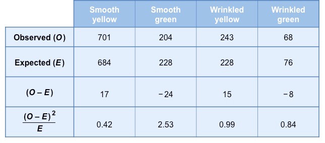
Create a table:
Phenotype Observed (O) Expected (E) \( (O - E)^2 \) \( \frac{(O - E)^2}{E} \) Tall 33 30 9 0.3 Short 7 10 9 0.9 Total 1.2 -
Calculate degrees of freedom: \( df = n - 1 = 2 - 1 = 1 \)
-
Determine chi-square value: \( \chi^2 = 1.2 \)
-
Compare with critical value: Using a chi-square distribution table, compare the calculated chi-square value with the critical value at 1 degree of freedom and a significance level of 0.05. If \( \chi^2 \) is less than the critical value (3.84), we accept the null hypothesis.
In this case, since 1.2 < 3.84, we accept the null hypothesis, indicating that the observed ratio fits the expected 3:1 ratio.
Chi-Square Table
| Degrees of Freedom | 0.9 | 0.5 | 0.1 | 0.05 | 0.01 |
| 1 | 0.02 | 0.46 | 2.71 | 3.84 | 6.64 |
| 2 | 0.21 | 1.39 | 4.61 | 5.99 | 9.21 |
| 3 | 0.58 | 2.37 | 6.25 | 7.82 | 11.35 |
| 4 | 1.06 | 3.36 | 7.78 | 9.49 | 13.28 |

READ MORE:
Introduction to Chi-Square Test in Genetics
The chi-square test is a statistical tool widely used in genetics to determine if there is a significant difference between observed and expected frequencies in categorical data. This test helps geneticists assess the goodness of fit between observed genetic data and theoretical genetic models.
In genetics, the chi-square test is often used to:
- Test Mendelian inheritance ratios
- Analyze inheritance patterns in organisms
- Verify Hardy-Weinberg equilibrium in populations
- Evaluate genetic linkage
The formula for the chi-square test is:
\[\chi^2 = \sum \frac{(O_i - E_i)^2}{E_i}\]
Where:
- \(O_i\) = Observed frequency
- \(E_i\) = Expected frequency
Steps to perform the chi-square test in genetics:
- State the null hypothesis \(H_0\): There is no significant difference between observed and expected frequencies.
- Calculate the expected frequencies based on the genetic hypothesis or model.
- Use the chi-square formula to compute the chi-square statistic.
- Determine the degrees of freedom (df): \(df = \text{number of categories} - 1\).
- Compare the calculated chi-square value to the critical value from the chi-square distribution table, based on the desired significance level (e.g., 0.05) and degrees of freedom.
- Make a decision: If the chi-square value is greater than the critical value, reject the null hypothesis; otherwise, do not reject it.
This test provides a way to objectively evaluate whether deviations from expected genetic ratios are due to random chance or indicate a significant difference, thus playing a crucial role in genetic research and analysis.
Understanding Mendelian Genetics
Mendelian genetics, founded by Gregor Mendel in the 19th century, forms the cornerstone of classical genetics. Mendel's experiments with pea plants established the fundamental laws of inheritance, which describe how traits are passed from parents to offspring.
Key concepts in Mendelian genetics include:
- Genes and Alleles: Genes are units of heredity, and alleles are different versions of a gene. Each individual inherits two alleles for each gene, one from each parent.
- Dominant and Recessive Alleles: Dominant alleles mask the effects of recessive alleles. An individual with at least one dominant allele will express the dominant trait.
- Homozygous and Heterozygous: An individual with two identical alleles for a gene is homozygous, while an individual with two different alleles is heterozygous.
Mendel's Laws of Inheritance:
- Law of Segregation: During the formation of gametes, the two alleles for a gene separate, so each gamete carries only one allele for each gene.
- Law of Independent Assortment: Alleles for different genes assort independently of one another during gamete formation, leading to genetic variation.
Using the chi-square test in Mendelian genetics involves comparing observed offspring ratios to expected ratios based on Mendelian laws. For example, in a monohybrid cross where one trait is studied, the expected phenotypic ratio for a heterozygous cross (Aa x Aa) is 3:1 (dominant to recessive).
Example Calculation:
Suppose a geneticist crosses two heterozygous pea plants (Aa x Aa) and observes the following offspring:
- 315 plants with dominant phenotype (A-)
- 85 plants with recessive phenotype (aa)
The expected ratio for a monohybrid cross is 3:1, so out of 400 offspring:
- Expected dominant phenotype = \( \frac{3}{4} \times 400 = 300 \)
- Expected recessive phenotype = \( \frac{1}{4} \times 400 = 100 \)
Using the chi-square formula:
\[\chi^2 = \frac{(315 - 300)^2}{300} + \frac{(85 - 100)^2}{100} = \frac{15^2}{300} + \frac{15^2}{100} = 0.75 + 2.25 = 3.0\]
Comparing this chi-square value with the critical value from the chi-square distribution table (with 1 degree of freedom at a 0.05 significance level), we can determine whether to accept or reject the null hypothesis that the observed data fits the expected Mendelian ratio.
Chi-Square Test Formula and Calculation
The chi-square test is a statistical method used to compare observed and expected frequencies in categorical data to determine if there is a significant difference between them. It is particularly useful in genetics for testing hypotheses about inheritance patterns and population genetics.
The formula for the chi-square test is:
\[\chi^2 = \sum \frac{(O_i - E_i)^2}{E_i}\]
Where:
- \(O_i\) = Observed frequency
- \(E_i\) = Expected frequency
Steps to perform the chi-square test:
- State the null hypothesis \(H_0\): There is no significant difference between the observed and expected frequencies.
- Calculate the expected frequencies: Based on the genetic model or hypothesis being tested, determine the expected frequencies for each category.
- Compute the chi-square statistic: Use the chi-square formula to calculate the chi-square value.
- Determine the degrees of freedom (df): The degrees of freedom are calculated as the number of categories minus one: \(df = \text{number of categories} - 1\).
- Compare the chi-square value: Find the critical value from the chi-square distribution table based on the desired significance level (e.g., 0.05) and degrees of freedom.
- Make a decision: If the chi-square value is greater than the critical value, reject the null hypothesis; otherwise, do not reject it.
Example Calculation:
Consider a genetic experiment with the following observed data for a monohybrid cross (Aa x Aa):
- Observed dominant phenotype (A-): 315
- Observed recessive phenotype (aa): 85
The expected ratio for a monohybrid cross is 3:1. For 400 offspring:
- Expected dominant phenotype: \( \frac{3}{4} \times 400 = 300 \)
- Expected recessive phenotype: \( \frac{1}{4} \times 400 = 100 \)
Using the chi-square formula:
\[\chi^2 = \frac{(315 - 300)^2}{300} + \frac{(85 - 100)^2}{100} = \frac{15^2}{300} + \frac{15^2}{100} = 0.75 + 2.25 = 3.0\]
With 1 degree of freedom (df = 2 - 1 = 1) and a significance level of 0.05, the critical value from the chi-square distribution table is approximately 3.841. Since the calculated chi-square value (3.0) is less than the critical value (3.841), we do not reject the null hypothesis. This indicates that the observed data fits the expected 3:1 ratio.
Example 1: Testing Mendelian Ratios
In this example, we will use the chi-square test to determine whether the observed ratios of offspring in a genetic cross fit the expected Mendelian ratios. We will consider a classic monohybrid cross involving a single gene with two alleles: dominant (A) and recessive (a).
Scenario: A geneticist crosses two heterozygous pea plants (Aa x Aa) and observes the following offspring:
- Observed dominant phenotype (A-): 315
- Observed recessive phenotype (aa): 85
The expected Mendelian ratio for a monohybrid cross (Aa x Aa) is 3:1 (dominant to recessive).
Step-by-Step Calculation:
- State the null hypothesis \(H_0\): The observed ratio of dominant to recessive phenotypes fits the expected 3:1 Mendelian ratio.
- Calculate the expected frequencies: Based on the expected 3:1 ratio, calculate the expected numbers of each phenotype for a total of 400 offspring:
- Expected dominant phenotype: \( \frac{3}{4} \times 400 = 300 \)
- Expected recessive phenotype: \( \frac{1}{4} \times 400 = 100 \)
- Compute the chi-square statistic: Use the chi-square formula:
\[\chi^2 = \frac{(315 - 300)^2}{300} + \frac{(85 - 100)^2}{100} = \frac{15^2}{300} + \frac{15^2}{100} = 0.75 + 2.25 = 3.0\]
- Determine the degrees of freedom (df): The degrees of freedom are calculated as the number of categories minus one: \(df = 2 - 1 = 1\).
- Compare the chi-square value: Find the critical value from the chi-square distribution table based on the desired significance level (e.g., 0.05) and degrees of freedom. For \(df = 1\) and \( \alpha = 0.05 \), the critical value is approximately 3.841.
- Make a decision: Compare the calculated chi-square value (3.0) to the critical value (3.841):
- If \(\chi^2 > \text{critical value}\), reject the null hypothesis.
- If \(\chi^2 \leq \text{critical value}\), do not reject the null hypothesis.
In this case, 3.0 is less than 3.841, so we do not reject the null hypothesis. This indicates that the observed data fits the expected 3:1 Mendelian ratio.
Thus, the chi-square test confirms that the observed ratios of offspring are consistent with Mendelian inheritance.
Example 2: Inheritance Patterns in Drosophila
In this example, we will use the chi-square test to analyze the inheritance patterns of a specific trait in Drosophila melanogaster (fruit flies). We will examine whether the observed ratios of offspring match the expected ratios based on a genetic hypothesis.
Scenario: A geneticist studies the inheritance of eye color in Drosophila, where red eyes (R) are dominant and white eyes (r) are recessive. A cross between heterozygous red-eyed flies (Rr x Rr) yields the following offspring:
- Observed red-eyed flies (R-): 580
- Observed white-eyed flies (rr): 220
The expected Mendelian ratio for this dihybrid cross (Rr x Rr) is 3:1 (red-eyed to white-eyed).
Step-by-Step Calculation:
- State the null hypothesis \(H_0\): The observed ratio of red-eyed to white-eyed flies fits the expected 3:1 ratio.
- Calculate the expected frequencies: Based on the expected 3:1 ratio, calculate the expected numbers of each phenotype for a total of 800 offspring:
- Expected red-eyed flies: \( \frac{3}{4} \times 800 = 600 \)
- Expected white-eyed flies: \( \frac{1}{4} \times 800 = 200 \)
- Compute the chi-square statistic: Use the chi-square formula:
\[\chi^2 = \frac{(580 - 600)^2}{600} + \frac{(220 - 200)^2}{200} = \frac{20^2}{600} + \frac{20^2}{200} = \frac{400}{600} + \frac{400}{200} = 0.67 + 2 = 2.67\]
- Determine the degrees of freedom (df): The degrees of freedom are calculated as the number of categories minus one: \(df = 2 - 1 = 1\).
- Compare the chi-square value: Find the critical value from the chi-square distribution table based on the desired significance level (e.g., 0.05) and degrees of freedom. For \(df = 1\) and \( \alpha = 0.05 \), the critical value is approximately 3.841.
- Make a decision: Compare the calculated chi-square value (2.67) to the critical value (3.841):
- If \(\chi^2 > \text{critical value}\), reject the null hypothesis.
- If \(\chi^2 \leq \text{critical value}\), do not reject the null hypothesis.
In this case, 2.67 is less than 3.841, so we do not reject the null hypothesis. This indicates that the observed data fits the expected 3:1 ratio.
Thus, the chi-square test confirms that the observed ratios of red-eyed and white-eyed flies are consistent with the expected Mendelian inheritance pattern.
Example 3: Hardy-Weinberg Equilibrium
In this example, we will use the chi-square test to determine whether a population is in Hardy-Weinberg equilibrium. The Hardy-Weinberg principle states that allele and genotype frequencies in a population will remain constant from generation to generation in the absence of evolutionary influences.
Scenario: A geneticist studies a population of 200 individuals to determine if the population is in Hardy-Weinberg equilibrium for a gene with two alleles: dominant (A) and recessive (a). The observed genotypes are:
- Observed AA: 90
- Observed Aa: 80
- Observed aa: 30
To test for Hardy-Weinberg equilibrium, we follow these steps:
- State the null hypothesis \(H_0\): The population is in Hardy-Weinberg equilibrium.
- Calculate allele frequencies:
- Frequency of allele A (p): \( p = \frac{2 \times \text{AA} + \text{Aa}}{2 \times \text{total individuals}} = \frac{2 \times 90 + 80}{2 \times 200} = \frac{260}{400} = 0.65 \)
- Frequency of allele a (q): \( q = \frac{2 \times \text{aa} + \text{Aa}}{2 \times \text{total individuals}} = \frac{2 \times 30 + 80}{2 \times 200} = \frac{140}{400} = 0.35 \)
Since \( p + q = 1 \), the calculations are correct.
- Calculate expected genotype frequencies: Using the Hardy-Weinberg formula:
- Expected frequency of AA: \( p^2 = 0.65^2 = 0.4225 \)
- Expected frequency of Aa: \( 2pq = 2 \times 0.65 \times 0.35 = 0.455 \)
- Expected frequency of aa: \( q^2 = 0.35^2 = 0.1225 \)
- Calculate expected genotype counts: Multiply the expected frequencies by the total number of individuals:
- Expected AA: \( 0.4225 \times 200 = 84.5 \)
- Expected Aa: \( 0.455 \times 200 = 91 \)
- Expected aa: \( 0.1225 \times 200 = 24.5 \)
- Compute the chi-square statistic: Use the chi-square formula:
\[\chi^2 = \frac{(90 - 84.5)^2}{84.5} + \frac{(80 - 91)^2}{91} + \frac{(30 - 24.5)^2}{24.5} = \frac{5.5^2}{84.5} + \frac{11^2}{91} + \frac{5.5^2}{24.5} = 0.36 + 1.33 + 1.23 = 2.92\]
- Determine the degrees of freedom (df): The degrees of freedom are calculated as the number of categories minus one: \(df = 3 - 1 = 2\).
- Compare the chi-square value: Find the critical value from the chi-square distribution table based on the desired significance level (e.g., 0.05) and degrees of freedom. For \(df = 2\) and \( \alpha = 0.05 \), the critical value is approximately 5.991.
- Make a decision: Compare the calculated chi-square value (2.92) to the critical value (5.991):
- If \(\chi^2 > \text{critical value}\), reject the null hypothesis.
- If \(\chi^2 \leq \text{critical value}\), do not reject the null hypothesis.
In this case, 2.92 is less than 5.991, so we do not reject the null hypothesis. This indicates that the population is in Hardy-Weinberg equilibrium for this gene.
Thus, the chi-square test confirms that the observed genotype frequencies are consistent with Hardy-Weinberg equilibrium.
Interpreting Chi-Square Test Results
Interpreting the results of a chi-square test involves comparing the calculated chi-square value to a critical value from the chi-square distribution table. Here is a step-by-step guide to interpreting the chi-square test results:
- Calculate the chi-square value:
Use the chi-square formula to calculate the chi-square value (\(\chi^2\)).
\[\chi^2 = \sum \frac{(O_i - E_i)^2}{E_i}\]
- Determine the degrees of freedom (df):
The degrees of freedom are calculated as the number of categories minus one:
\[df = \text{number of categories} - 1\]
- Select a significance level (\(\alpha\)):
The significance level is typically set at 0.05 (5%), but other values such as 0.01 or 0.10 can also be used.
- Find the critical value:
Use the chi-square distribution table to find the critical value corresponding to the degrees of freedom and the selected significance level.
Degrees of Freedom (df) Critical Value (\(\alpha = 0.05\)) Critical Value (\(\alpha = 0.01\)) 1 3.841 6.635 2 5.991 9.210 3 7.815 11.345 4 9.488 13.277 - Compare the chi-square value to the critical value:
- If \(\chi^2 > \text{critical value}\), reject the null hypothesis.
- If \(\chi^2 \leq \text{critical value}\), do not reject the null hypothesis.
- Interpret the results:
- Rejecting the null hypothesis indicates that there is a significant difference between the observed and expected frequencies, suggesting that the observed data does not fit the expected distribution.
- Not rejecting the null hypothesis indicates that there is no significant difference between the observed and expected frequencies, suggesting that the observed data fits the expected distribution.
Example Interpretation:
In an experiment testing the inheritance pattern in Drosophila, the calculated chi-square value is 2.67 with 1 degree of freedom and a significance level of 0.05. The critical value from the chi-square distribution table is 3.841.
- Since 2.67 is less than 3.841, we do not reject the null hypothesis.
- This indicates that the observed data fits the expected Mendelian ratio, and there is no significant difference between the observed and expected frequencies.
Chi-Square Test for Multiple Alleles
The chi-square test can also be used to analyze inheritance patterns involving multiple alleles. In this example, we will determine whether the observed frequencies of different blood types in a population fit the expected ratios based on known genetic inheritance.
Scenario: A geneticist examines the blood types (A, B, AB, and O) of 300 individuals to determine if the observed distribution matches the expected frequencies based on the Hardy-Weinberg equilibrium for multiple alleles (IA, IB, and i).
- Observed blood type A: 120
- Observed blood type B: 90
- Observed blood type AB: 30
- Observed blood type O: 60
The expected frequencies for blood types in a population are calculated based on allele frequencies (p for IA, q for IB, and r for i).
Step-by-Step Calculation:
- State the null hypothesis \(H_0\): The observed blood type frequencies fit the expected distribution based on the Hardy-Weinberg equilibrium.
- Calculate allele frequencies: Let's assume the allele frequencies are:
- Frequency of IA (p): 0.3
- Frequency of IB (q): 0.2
- Frequency of i (r): 0.5
- Calculate expected genotype frequencies: Using the Hardy-Weinberg formula for multiple alleles:
- Expected frequency of blood type A (IAIA + IAi): \( p^2 + 2pr = 0.3^2 + 2 \times 0.3 \times 0.5 = 0.09 + 0.3 = 0.39 \)
- Expected frequency of blood type B (IBIB + IBi): \( q^2 + 2qr = 0.2^2 + 2 \times 0.2 \times 0.5 = 0.04 + 0.2 = 0.24 \)
- Expected frequency of blood type AB (IAIB): \( 2pq = 2 \times 0.3 \times 0.2 = 0.12 \)
- Expected frequency of blood type O (ii): \( r^2 = 0.5^2 = 0.25 \)
- Calculate expected genotype counts: Multiply the expected frequencies by the total number of individuals (300):
- Expected blood type A: \( 0.39 \times 300 = 117 \)
- Expected blood type B: \( 0.24 \times 300 = 72 \)
- Expected blood type AB: \( 0.12 \times 300 = 36 \)
- Expected blood type O: \( 0.25 \times 300 = 75 \)
- Compute the chi-square statistic: Use the chi-square formula:
\[\chi^2 = \sum \frac{(O_i - E_i)^2}{E_i}\]
\[\chi^2 = \frac{(120 - 117)^2}{117} + \frac{(90 - 72)^2}{72} + \frac{(30 - 36)^2}{36} + \frac{(60 - 75)^2}{75} = \frac{3^2}{117} + \frac{18^2}{72} + \frac{6^2}{36} + \frac{15^2}{75} = 0.077 + 4.5 + 1 + 3 = 8.577\]
- Determine the degrees of freedom (df): The degrees of freedom are calculated as the number of categories minus one: \(df = 4 - 1 = 3\).
- Compare the chi-square value: Find the critical value from the chi-square distribution table based on the desired significance level (e.g., 0.05) and degrees of freedom. For \(df = 3\) and \( \alpha = 0.05 \), the critical value is approximately 7.815.
- Make a decision: Compare the calculated chi-square value (8.577) to the critical value (7.815):
- If \(\chi^2 > \text{critical value}\), reject the null hypothesis.
- If \(\chi^2 \leq \text{critical value}\), do not reject the null hypothesis.
In this case, 8.577 is greater than 7.815, so we reject the null hypothesis. This indicates that the observed data does not fit the expected distribution based on Hardy-Weinberg equilibrium.
Thus, the chi-square test suggests that the observed blood type frequencies in the population do not conform to the expected frequencies under Hardy-Weinberg equilibrium for multiple alleles.

Application of Chi-Square Test in Human Genetics
The chi-square test is widely used in human genetics to determine if observed genetic data fits expected ratios based on genetic inheritance patterns. This test helps in understanding how genes are transmitted from parents to offspring and can be applied to various genetic scenarios.
Example Scenario: A study is conducted to determine if the distribution of blood types in a population follows the expected genetic ratios. The blood types are A, B, AB, and O, inherited through multiple alleles (IA, IB, and i).
- Observed blood type A: 150
- Observed blood type B: 100
- Observed blood type AB: 50
- Observed blood type O: 200
To apply the chi-square test in this context, follow these steps:
- State the null hypothesis \(H_0\): The observed distribution of blood types fits the expected distribution based on genetic inheritance.
- Calculate allele frequencies:
- Frequency of IA (p): 0.3
- Frequency of IB (q): 0.2
- Frequency of i (r): 0.5
- Calculate expected genotype frequencies: Using Hardy-Weinberg equilibrium for multiple alleles:
- Expected frequency of blood type A (IAIA + IAi): \( p^2 + 2pr = 0.3^2 + 2 \times 0.3 \times 0.5 = 0.09 + 0.3 = 0.39 \)
- Expected frequency of blood type B (IBIB + IBi): \( q^2 + 2qr = 0.2^2 + 2 \times 0.2 \times 0.5 = 0.04 + 0.2 = 0.24 \)
- Expected frequency of blood type AB (IAIB): \( 2pq = 2 \times 0.3 \times 0.2 = 0.12 \)
- Expected frequency of blood type O (ii): \( r^2 = 0.5^2 = 0.25 \)
- Calculate expected genotype counts: Multiply the expected frequencies by the total number of individuals (500):
- Expected blood type A: \( 0.39 \times 500 = 195 \)
- Expected blood type B: \( 0.24 \times 500 = 120 \)
- Expected blood type AB: \( 0.12 \times 500 = 60 \)
- Expected blood type O: \( 0.25 \times 500 = 125 \)
- Compute the chi-square statistic: Use the chi-square formula:
\[\chi^2 = \sum \frac{(O_i - E_i)^2}{E_i}\]
\[\chi^2 = \frac{(150 - 195)^2}{195} + \frac{(100 - 120)^2}{120} + \frac{(50 - 60)^2}{60} + \frac{(200 - 125)^2}{125} = \frac{45^2}{195} + \frac{20^2}{120} + \frac{10^2}{60} + \frac{75^2}{125} = 10.385 + 3.333 + 1.667 + 45 = 60.385\]
- Determine the degrees of freedom (df): The degrees of freedom are calculated as the number of categories minus one: \(df = 4 - 1 = 3\).
- Compare the chi-square value: Find the critical value from the chi-square distribution table based on the desired significance level (e.g., 0.05) and degrees of freedom. For \(df = 3\) and \( \alpha = 0.05 \), the critical value is approximately 7.815.
- Make a decision: Compare the calculated chi-square value (60.385) to the critical value (7.815):
- If \(\chi^2 > \text{critical value}\), reject the null hypothesis.
- If \(\chi^2 \leq \text{critical value}\), do not reject the null hypothesis.
In this case, 60.385 is greater than 7.815, so we reject the null hypothesis. This indicates that the observed distribution of blood types does not fit the expected genetic distribution.
Thus, the chi-square test can be effectively used to analyze and interpret genetic data in human populations, providing insights into inheritance patterns and potential deviations from expected genetic distributions.
Common Pitfalls and Misinterpretations
The chi-square test is a powerful tool in genetics, but its proper application requires careful attention to detail. Here are some common pitfalls and misinterpretations to avoid:
- Small Sample Sizes: The chi-square test requires a sufficiently large sample size to provide accurate results. If the expected frequency in any category is less than 5, the test might not be valid. In such cases, consider using an exact test instead.
- Incorrect Application of the Test: The chi-square test is designed for categorical data. Applying it to continuous data or data that do not fit into discrete categories can lead to erroneous conclusions.
- Misinterpreting the P-value: A common mistake is to misinterpret the P-value. A P-value greater than 0.05 does not prove that the null hypothesis is true; it merely indicates that there is not enough evidence to reject it. Conversely, a P-value less than 0.05 suggests that there is a significant difference, but it does not quantify the magnitude of this difference.
- Ignoring the Assumptions: The chi-square test has specific assumptions, including the independence of observations and the adequacy of sample size. Violating these assumptions can lead to misleading results.
- Overlooking Effect Size: While the chi-square test can tell you whether a difference exists, it does not indicate the size or importance of that difference. Reporting effect size along with the chi-square statistic provides a more complete picture.
- Incorrect Degrees of Freedom: Calculating the degrees of freedom incorrectly is a common error. The degrees of freedom for a chi-square test are determined by the number of categories minus one (for a goodness-of-fit test) or the product of the number of categories in each variable minus one (for a test of independence).
- Combining Categories Inappropriately: Sometimes, researchers combine categories to meet the assumptions of the chi-square test. This can be problematic if it distorts the data or the relationships within it. Each combination should be justifiable and based on sound reasoning.
- Post-Hoc Testing without Adjustment: Performing multiple chi-square tests on the same dataset increases the risk of Type I errors (false positives). Adjustments, such as the Bonferroni correction, should be made to account for multiple comparisons.
By carefully considering these pitfalls and ensuring the correct application of the chi-square test, researchers can avoid common mistakes and derive more accurate conclusions from their genetic data.
Conclusion and Further Reading
The Chi-Square test is a powerful statistical tool used extensively in genetics to determine if there is a significant association between observed and expected frequencies. It aids in verifying hypotheses related to genetic crosses, inheritance patterns, and population genetics.
Through various examples, such as testing Mendelian ratios, analyzing inheritance patterns in Drosophila, and assessing Hardy-Weinberg equilibrium, we have seen how the Chi-Square test can provide insights into genetic phenomena. However, it is crucial to apply the test correctly and be mindful of its assumptions and limitations to avoid common pitfalls and misinterpretations.
In summary, the Chi-Square test offers a robust method for analyzing categorical data in genetics. By understanding its principles and carefully interpreting the results, researchers can draw meaningful conclusions about genetic patterns and inheritance.
Further Reading
Tìm hiểu về kiểm tra Chi-Square và các ví dụ về lai giống di truyền trong video này. Phù hợp với từ khóa 'chi square test example genetics'.
Kiểm Tra Chi-Square và Lai Giống Di Truyền
READ MORE:
Khám phá kiểm tra Chi-Square và các vấn đề di truyền qua video này. Phù hợp với từ khóa 'chi square test example genetics'.
Kiểm Tra Chi-Square và Các Vấn Đề Di Truyền

:max_bytes(150000):strip_icc()/Chi-SquareStatistic_Final_4199464-7eebcd71a4bf4d9ca1a88d278845e674.jpg)