Topic examples of chi-square test for independence: Explore compelling examples of the Chi-Square Test for Independence and learn how this statistical tool uncovers relationships between categorical variables. From gender voting patterns to snack preferences at the movies, discover how the Chi-Square test helps identify significant associations and insights across diverse datasets.
Table of Content
- Examples of Chi-Square Test for Independence
- Introduction to Chi-Square Test for Independence
- Understanding the Chi-Square Distribution
- Basic Principles and Assumptions of the Test
- Step-by-Step Process of Conducting the Test
- Calculating Expected Frequencies
- Interpreting Chi-Square Results
- Examples and Applications
- 4. Customer Satisfaction and Product Type
- Common Mistakes and How to Avoid Them
- Real-World Case Studies
- Statistical Software for Chi-Square Tests
- Advantages and Limitations of the Test
- Chi-Square Test for Independence vs. Chi-Square Goodness of Fit
- FAQs and Troubleshooting
- Conclusion and Further Reading
- YOUTUBE: Video về Phân tích Chi-Square cho Sự Độc Lập, hướng dẫn cụ thể và ứng dụng trong nghiên cứu.
Examples of Chi-Square Test for Independence
The Chi-Square Test for Independence is a statistical method used to determine if there is a significant association between two categorical variables. Below are some detailed examples and explanations to help you understand how to apply this test in various scenarios.
1. Gender and Voting Preference
Suppose we want to test if there is an association between gender and voting preference in an election. We collect data from a random sample of voters and organize it into a contingency table:
| Republican | Democrat | Independent | Total | |
| Male | 120 | 90 | 40 | 250 |
| Female | 110 | 95 | 45 | 250 |
| Total | 230 | 185 | 85 | 500 |
To test for independence, we calculate the expected frequencies for each cell under the assumption that gender and voting preference are independent. Using the formula:
\[
\text{Expected Frequency} = \frac{(\text{Row Total} \times \text{Column Total})}{\text{Grand Total}}
\]
For instance, the expected frequency for Male Republicans is calculated as:
\[
\text{Expected} = \frac{(250 \times 230)}{500} = 115
\]
We then perform similar calculations for all cells, and compare the observed frequencies with these expected frequencies to compute the Chi-Square statistic.
2. Movie Genre and Snack Preference
Consider a study to determine if there is a relationship between movie genre preference and the type of snack purchased. The data collected is presented as follows:
| Popcorn | Candy | No Snacks | Total | |
| Action | 50 | 65 | 10 | 125 |
| Comedy | 75 | 80 | 45 | 200 |
| Drama | 60 | 40 | 20 | 120 |
| Total | 185 | 185 | 75 | 445 |
Again, we calculate the expected counts for each cell. For example, for the Action-Popcorn cell, the expected count is:
\[
\text{Expected} = \frac{(125 \times 185)}{445} \approx 52.25
\]
We then use these expected counts to compute the Chi-Square statistic and determine if there is a significant relationship between movie genre and snack preference.
3. Educational Level and Internet Usage
A survey investigates if educational level affects the frequency of internet usage. The collected data is summarized below:
| Never | Occasionally | Frequently | Total | |
| High School | 30 | 40 | 30 | 100 |
| Bachelor's | 20 | 50 | 60 | 130 |
| Master's | 10 | 30 | 60 | 100 |
| Total | 60 | 120 | 150 | 330 |
Expected counts are calculated, such as for High School students who use the internet occasionally:
\[
\text{Expected} = \frac{(100 \times 120)}{330} \approx 36.36
\]
By comparing the observed and expected frequencies, we can use the Chi-Square test to assess whether internet usage is independent of educational level.
4. Conclusion
These examples illustrate how the Chi-Square Test for Independence can be applied to different types of categorical data to test for associations. By comparing observed data with expected data under the assumption of independence, we can make informed decisions about the relationships between variables.

READ MORE:
Introduction to Chi-Square Test for Independence
The Chi-Square Test for Independence is a fundamental statistical tool used to determine whether there is a significant association between two categorical variables. This non-parametric test is particularly useful in fields such as social sciences, marketing, and biology, where understanding the relationship between variables can lead to important insights. Below is a step-by-step guide to understanding and applying this test:
- Purpose: The primary goal of the Chi-Square Test for Independence is to assess whether two variables are independent or if there is a significant relationship between them.
- Applications: It is commonly used to analyze survey data, experiment results, and observational studies where data is categorized into groups.
Step-by-Step Guide to Conducting the Chi-Square Test for Independence
- Set Up the Hypotheses:
- Null Hypothesis (\(H_0\)): Assumes that there is no association between the two variables; they are independent.
- Alternative Hypothesis (\(H_1\)): Assumes that there is an association between the variables; they are not independent.
- Create a Contingency Table:
Organize the data into a table where rows represent one variable and columns represent the other. Each cell in the table shows the frequency count of occurrences for the specific combination of variables.
Variable B1 Variable B2 Total Variable A1 Count Count Row Total Variable A2 Count Count Row Total Total Column Total Column Total Grand Total - Calculate the Expected Frequencies:
For each cell in the contingency table, calculate the expected frequency assuming that the variables are independent. The formula is:
\[
\text{Expected Frequency} = \frac{(\text{Row Total} \times \text{Column Total})}{\text{Grand Total}}
\] - Compute the Chi-Square Statistic:
Compare the observed and expected frequencies using the formula:
\[
\chi^2 = \sum \frac{(O_i - E_i)^2}{E_i}
\]where \(O_i\) is the observed frequency, and \(E_i\) is the expected frequency for each cell.
- Determine the Degrees of Freedom:
The degrees of freedom (\(df\)) for the test are calculated as:
\[
df = (r - 1) \times (c - 1)
\]where \(r\) is the number of rows and \(c\) is the number of columns in the contingency table.
- Find the Critical Value and Make a Decision:
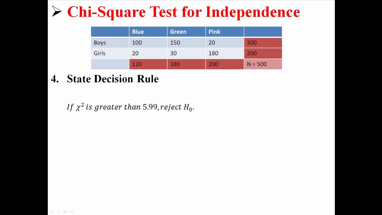
Using the Chi-Square distribution table, find the critical value for the given significance level (\(\alpha\)) and degrees of freedom. Compare the Chi-Square statistic to the critical value:
- If \(\chi^2\) is greater than the critical value, reject the null hypothesis (\(H_0\)), indicating a significant association between the variables.
- If \(\chi^2\) is less than or equal to the critical value, fail to reject the null hypothesis, suggesting no significant association.
The Chi-Square Test for Independence provides a robust method for exploring relationships in categorical data, helping researchers and analysts uncover hidden patterns and associations.
Understanding the Chi-Square Distribution
The Chi-Square distribution is a critical component in many statistical tests, including the Chi-Square Test for Independence. This distribution is essential for evaluating how well an observed data distribution fits with an expected distribution, especially when dealing with categorical data. Let's delve into the key aspects of the Chi-Square distribution:
- Definition: The Chi-Square distribution is a continuous probability distribution that describes the distribution of a sum of squared standard normal deviates. It is characterized by its degrees of freedom (\(df\)), which determine its shape.
- Degrees of Freedom:
The degrees of freedom in a Chi-Square distribution are related to the number of categories in the data. For a Chi-Square Test for Independence, the degrees of freedom are calculated as:
\[
df = (r - 1) \times (c - 1)
\]where \(r\) is the number of rows and \(c\) is the number of columns in the contingency table.
Properties of the Chi-Square Distribution
- Skewness: The Chi-Square distribution is positively skewed, meaning it has a long right tail. However, as the degrees of freedom increase, the distribution becomes more symmetric.
- Mean and Variance:
- The mean of a Chi-Square distribution is equal to the degrees of freedom (\(df\)).
- The variance is twice the degrees of freedom (\(2 \times df\)).
- Shape: The shape of the Chi-Square distribution changes with the degrees of freedom:
- For \(df = 1\), the distribution is highly skewed to the right.
- As \(df\) increases, the distribution approaches a normal distribution.
Below is a table summarizing the characteristics of the Chi-Square distribution for different degrees of freedom:
| Degrees of Freedom (\(df\)) | Mean | Variance | Shape |
|---|---|---|---|
| 1 | 1 | 2 | Highly skewed to the right |
| 5 | 5 | 10 | Moderately skewed to the right |
| 10 | 10 | 20 | Less skewed, closer to normal |
| 30 | 30 | 60 | Approximately normal |
Using the Chi-Square Distribution in Hypothesis Testing
When performing a Chi-Square Test for Independence, the Chi-Square distribution is used to determine the probability of observing the calculated Chi-Square statistic under the null hypothesis. This probability, known as the p-value, helps in deciding whether to reject the null hypothesis:
- Calculate the Chi-Square Statistic: Sum the squared differences between observed (\(O\)) and expected (\(E\)) frequencies, divided by the expected frequencies:
\[
\chi^2 = \sum \frac{(O_i - E_i)^2}{E_i}
\] - Find the p-value: Using the calculated Chi-Square statistic and the degrees of freedom, locate the corresponding p-value in the Chi-Square distribution table.
- Compare with the Significance Level: If the p-value is less than the chosen significance level (\(\alpha\)), reject the null hypothesis, indicating a significant association between the variables.
The Chi-Square distribution plays a pivotal role in hypothesis testing, providing a framework to assess the independence and relationship between categorical variables. Understanding its properties and applications is crucial for effectively utilizing the Chi-Square Test for Independence.
Basic Principles and Assumptions of the Test
The Chi-Square Test for Independence is used to determine if there is a significant association between two categorical variables. Understanding the basic principles and assumptions behind this test is crucial for its proper application and interpretation. Below, we explore these core elements in detail:
Principles of the Chi-Square Test for Independence
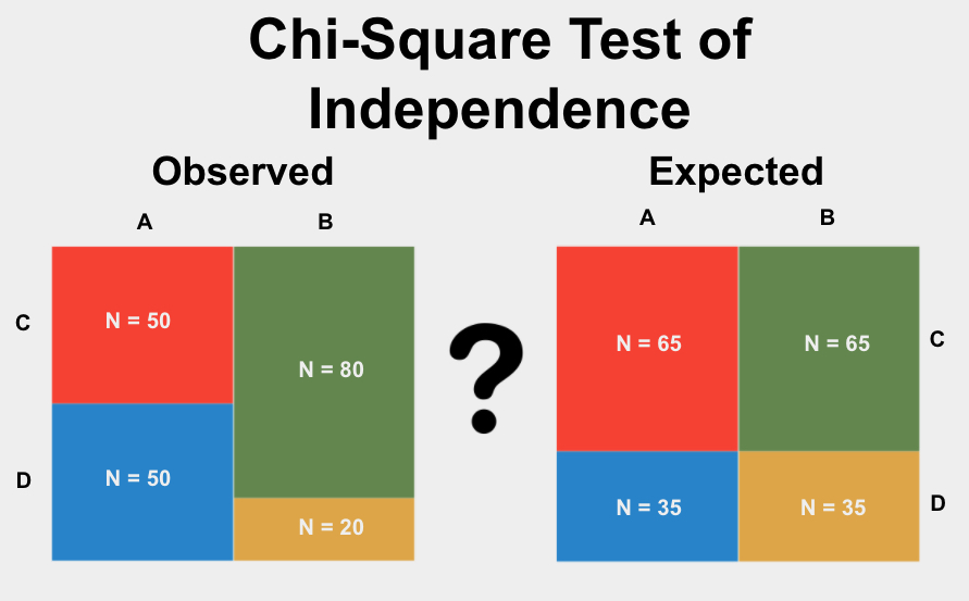
- Objective: The test aims to assess whether the observed frequencies in a contingency table differ significantly from the expected frequencies under the assumption that the variables are independent.
- Comparison of Observed and Expected Frequencies: It involves comparing the actual data (observed frequencies) with the data we would expect if the variables were independent (expected frequencies).
- Chi-Square Statistic: The Chi-Square (\(\chi^2\)) statistic is calculated using the formula:
\[
\chi^2 = \sum \frac{(O_i - E_i)^2}{E_i}
\]
where \(O_i\) represents the observed frequency and \(E_i\) the expected frequency for each cell in the contingency table. - Degrees of Freedom: The degrees of freedom for the test are determined by the number of rows and columns in the contingency table, calculated as:
\[
df = (r - 1) \times (c - 1)
\]
where \(r\) is the number of rows and \(c\) is the number of columns. - P-Value: The p-value indicates the probability that the observed distribution is due to chance. A lower p-value suggests a significant association between the variables.
Assumptions of the Chi-Square Test for Independence
- Independence of Observations: Each observation should be independent of all others. The test is not suitable for paired or related samples.
- Random Sampling: Data should be collected through random sampling to ensure that the results are representative of the population.
- Expected Frequency Threshold: Each cell in the contingency table should have an expected frequency of at least 5. If this condition is not met, the test may not be valid, and other methods or adjustments might be necessary.
- Categorical Data: The test is designed for categorical data, where variables represent categories rather than continuous or ordinal data.
- Mutually Exclusive Categories: The categories in the contingency table should be mutually exclusive, meaning an observation can only belong to one category in each variable.
Steps to Verify Assumptions
- Check Independence: Ensure that the data points are independent. This can be verified by confirming that each observation was recorded only once and does not influence others.
- Confirm Random Sampling: Review the data collection process to verify that the sample was randomly selected from the population.
- Calculate Expected Frequencies: Before performing the test, calculate the expected frequencies to ensure they meet the threshold of at least 5 per cell. This can be done using the formula:
\[
E_{ij} = \frac{(Row_i \times Column_j)}{N}
\]
where \(E_{ij}\) is the expected frequency for cell \(ij\), \(Row_i\) and \(Column_j\) are the totals for the \(i\)th row and \(j\)th column, and \(N\) is the grand total.
Understanding these principles and assumptions is vital for effectively applying the Chi-Square Test for Independence. Ensuring that your data meets these criteria will enhance the reliability and validity of your results.
Step-by-Step Process of Conducting the Test
The Chi-Square Test for Independence is a straightforward yet powerful method to determine if there is a significant association between two categorical variables. Follow these detailed steps to conduct the test effectively:
- Formulate Hypotheses:
- Null Hypothesis (\(H_0\)): Assumes that the variables are independent (no association exists).
- Alternative Hypothesis (\(H_1\)): Assumes that the variables are not independent (an association exists).
- Create a Contingency Table:
Organize your data into a contingency table where rows represent one categorical variable and columns represent the other. Each cell in the table shows the frequency count of occurrences for each combination of categories.
Category B1 Category B2 Category B3 Total Category A1 Count Count Count Row Total Category A2 Count Count Count Row Total Category A3 Count Count Count Row Total Total Column Total Column Total Column Total Grand Total - Calculate Expected Frequencies:
Determine the expected frequency for each cell in the contingency table using the formula:
\[
E_{ij} = \frac{(Row_i \times Column_j)}{N}
\]
where \(E_{ij}\) is the expected frequency for cell \(ij\), \(Row_i\) is the total count for row \(i\), \(Column_j\) is the total count for column \(j\), and \(N\) is the grand total of all observations. - Compute the Chi-Square Statistic:
Use the observed and expected frequencies to calculate the Chi-Square statistic (\(\chi^2\)) with the formula:
\[
\chi^2 = \sum \frac{(O_i - E_i)^2}{E_i}
\]
where \(O_i\) is the observed frequency and \(E_i\) is the expected frequency for each cell. - Determine Degrees of Freedom:
The degrees of freedom (\(df\)) for the test are calculated as:
\[
df = (r - 1) \times (c - 1)
\]
where \(r\) is the number of rows and \(c\) is the number of columns in the contingency table. - Find the Critical Value:
Using a Chi-Square distribution table, find the critical value that corresponds to your degrees of freedom and the chosen significance level (\(\alpha\)). This value is the threshold for determining statistical significance.
- Compare and Interpret the Results:
Compare the calculated Chi-Square statistic to the critical value:
- If \(\chi^2\) is greater than the critical value, reject the null hypothesis (\(H_0\)). This indicates a significant association between the variables.
- If \(\chi^2\) is less than or equal to the critical value, fail to reject the null hypothesis, suggesting no significant association.
- Report the Findings:
Summarize the results, including the Chi-Square statistic, degrees of freedom, p-value, and your conclusion regarding the independence of the variables.
By following these steps, you can effectively apply the Chi-Square Test for Independence to determine the relationship between categorical variables and gain valuable insights from your data.
Calculating Expected Frequencies
In the Chi-Square Test for Independence, calculating expected frequencies is a crucial step. These expected frequencies represent what we would anticipate in each cell of the contingency table if the two variables were truly independent. Here's a detailed step-by-step process for calculating the expected frequencies:
Steps to Calculate Expected Frequencies
- Create a Contingency Table:
Begin by organizing your observed data into a contingency table. Each cell in the table represents the frequency count of occurrences for each combination of the categories of the two variables.
Category B1 Category B2 Category B3 Total Category A1 O11 O12 O13 Row Total A1 Category A2 O21 O22 O23 Row Total A2 Category A3 O31 O32 O33 Row Total A3 Total Column Total B1 Column Total B2 Column Total B3 Grand Total In this table, \(O_{ij}\) represents the observed frequency in the cell at row \(i\) and column \(j\).
- Calculate Row and Column Totals:
Sum the frequencies for each row and each column. These totals will be used to calculate the expected frequencies. The grand total is the sum of all observations in the table.
- Row Totals: Sum the counts across each row.
- Column Totals: Sum the counts down each column.
- Grand Total: Sum of all the row totals or column totals (they should be the same).
- Compute Expected Frequencies:
The expected frequency for each cell (\(E_{ij}\)) is calculated using the formula:
\[
E_{ij} = \frac{(Row_i \times Column_j)}{N}
\]where:
- \(E_{ij}\) = expected frequency for cell in row \(i\) and column \(j\).
- Rowi = total count for row \(i\).
- Columnj = total count for column \(j\).
- \(N\) = grand total (sum of all observed frequencies).
Let's apply this to the example table:
Category B1 Category B2 Category B3 Total Category A1 \(E_{11} = \frac{(Row\_Total\_A1 \times Col\_Total\_B1)}{N}\) \(E_{12} = \frac{(Row\_Total\_A1 \times Col\_Total\_B2)}{N}\) \(E_{13} = \frac{(Row\_Total\_A1 \times Col\_Total\_B3)}{N}\) Row Total A1 Category A2 \(E_{21} = \frac{(Row\_Total\_A2 \times Col\_Total\_B1)}{N}\) \(E_{22} = \frac{(Row\_Total\_A2 \times Col\_Total\_B2)}{N}\) \(E_{23} = \frac{(Row\_Total\_A2 \times Col\_Total\_B3)}{N}\) Row Total A2 Category A3 \(E_{31} = \frac{(Row\_Total\_A3 \times Col\_Total\_B1)}{N}\) \(E_{32} = \frac{(Row\_Total\_A3 \times Col\_Total\_B2)}{N}\) \(E_{33} = \frac{(Row\_Total\_A3 \times Col\_Total\_B3)}{N}\) Row Total A3 Total Column Total B1 Column Total B2 Column Total B3 Grand Total - Verify Expected Frequencies:
Ensure that all expected frequencies are at least 5. If any expected frequency is below this threshold, the validity of the Chi-Square test might be compromised, and you may need to use an alternative method or combine categories.
By following these steps, you can accurately calculate the expected frequencies necessary for performing the Chi-Square Test for Independence, ensuring your analysis is both valid and reliable.
Interpreting Chi-Square Results
After conducting the Chi-Square Test for Independence, the next crucial step is interpreting the results. This involves understanding the Chi-Square statistic, degrees of freedom, p-value, and how these elements determine the relationship between the variables. Here’s a detailed guide on how to interpret Chi-Square test results:
Key Components to Understand
- Chi-Square Statistic (\(\chi^2\)):
This value quantifies the difference between the observed and expected frequencies. It is calculated using the formula:
\[
\chi^2 = \sum \frac{(O_i - E_i)^2}{E_i}
\]
where \(O_i\) is the observed frequency and \(E_i\) is the expected frequency for each cell.A higher Chi-Square value indicates a larger discrepancy between the observed and expected frequencies, suggesting a stronger association between the variables.
- Degrees of Freedom (df):
The degrees of freedom in a Chi-Square test are calculated as:
\[
df = (r - 1) \times (c - 1)
\]
where \(r\) is the number of rows and \(c\) is the number of columns in the contingency table.Degrees of freedom reflect the number of values that are free to vary while calculating the Chi-Square statistic. This is important for determining the critical value from the Chi-Square distribution table.
- P-Value:
The p-value represents the probability of observing the given data, or something more extreme, assuming the null hypothesis is true. It is compared against a significance level (\(\alpha\)), typically 0.05 or 0.01.
- If \(p \leq \alpha\), reject the null hypothesis (\(H_0\)). This indicates a significant association between the variables.
- If \(p > \alpha\), fail to reject the null hypothesis. This suggests no significant association between the variables.
The smaller the p-value, the stronger the evidence against the null hypothesis.
- Critical Value:
Using the Chi-Square distribution table, find the critical value corresponding to your calculated degrees of freedom and chosen significance level. The critical value serves as a threshold for determining the statistical significance of your test.
Steps to Interpret the Results
- Calculate the Chi-Square Statistic:
Compute the Chi-Square statistic based on your observed and expected frequencies.
- Determine the Degrees of Freedom:
Calculate the degrees of freedom for your contingency table.
- Find the Critical Value:
Use the Chi-Square distribution table to find the critical value for your degrees of freedom and chosen significance level.
- Compare the Chi-Square Statistic to the Critical Value:
Assess whether your calculated Chi-Square statistic exceeds the critical value.
- If \(\chi^2 > \text{critical value}\), reject the null hypothesis (\(H_0\)). There is a significant association between the variables.
- If \(\chi^2 \leq \text{critical value}\), fail to reject the null hypothesis. There is no significant association between the variables.
- Evaluate the P-Value:
Alternatively, you can evaluate the p-value associated with the Chi-Square statistic. Compare this p-value to your chosen significance level (\(\alpha\)).
- Draw Conclusions:
Summarize your findings based on the comparison of the Chi-Square statistic to the critical value or the p-value to the significance level. Clearly state whether there is evidence to suggest a significant association between the variables.
Interpreting the results of a Chi-Square Test for Independence allows researchers to understand the relationship between categorical variables in their data. By following these steps, you can draw meaningful conclusions and gain insights from your Chi-Square analysis.
Examples and Applications
Here are some practical examples illustrating the application of the Chi-Square Test for Independence:
-
Gender and Voting Preference:
A study examines whether there is an association between gender and voting preference among a sample of voters. The null hypothesis suggests that gender and voting preference are independent.
Republican Democrat Independent Male 210 180 60 Female 180 220 70 The Chi-Square Test for Independence assesses whether the observed frequencies (above) differ significantly from what would be expected under the assumption of independence.
-
Movie Genre and Snack Preference:
An entertainment survey investigates whether there is a relationship between movie genre preference and snack choice among cinema-goers.
Popcorn Candy Soda Action 120 80 60 Comedy 100 120 40 Drama 80 60 30 The Chi-Square Test determines whether there is a significant association between movie genre and snack preference.
-
Educational Level and Internet Usage:
A study explores the relationship between educational level and internet usage habits among a group of college students.
Heavy Usage Moderate Usage Light Usage High School 80 50 20 Undergraduate 120 100 40 Graduate 50 30 10 The Chi-Square Test evaluates whether there is a statistically significant relationship between educational level and internet usage patterns.
-
Customer Satisfaction and Product Type:
An industry survey investigates whether customer satisfaction levels vary significantly by product type.
Product A Product B Product C Satisfied 150 120 80 Neutral 50 80 40 Not Satisfied 30 40 20 The Chi-Square Test assesses whether there is a significant association between customer satisfaction and the type of product purchased.
4. Customer Satisfaction and Product Type
An industry survey investigates whether customer satisfaction levels vary significantly by product type.
| Product A | Product B | Product C | |
| Satisfied | 150 | 120 | 80 |
| Neutral | 50 | 80 | 40 |
| Not Satisfied | 30 | 40 | 20 |
The Chi-Square Test assesses whether there is a significant association between customer satisfaction and the type of product purchased.
Common Mistakes and How to Avoid Them
Incorrect application of the Chi-Square Test: Ensure that the test is used appropriately for categorical data analysis, specifically for testing independence or homogeneity.
Small sample sizes: Avoid drawing conclusions from Chi-Square tests with small sample sizes, as they may not provide reliable results.
Ignoring assumptions: Validate assumptions such as expected cell frequencies and independence of observations before conducting the test.
Confusing Chi-Square Test types: Differentiate between Chi-Square Test for Independence and Chi-Square Goodness of Fit, as they address different hypotheses.
Incorrect interpretation of results: Ensure clear understanding of Chi-Square test statistics and p-values to correctly interpret whether associations are statistically significant.
Real-World Case Studies
-
Healthcare and Patient Outcomes: Researchers investigate whether there is a relationship between the type of treatment received and recovery outcomes among patients.
Improved No Change Declined Treatment A 120 80 30 Treatment B 100 90 25 Treatment C 80 70 20 The Chi-Square Test examines whether the type of treatment significantly influences patient outcomes.
-
Marketing Campaign Effectiveness: A marketing firm analyzes the impact of different advertising strategies on customer engagement and brand perception.
High Engagement Moderate Engagement Low Engagement Strategy A 150 100 50 Strategy B 130 110 40 Strategy C 120 90 30 The Chi-Square Test assesses whether there is a statistically significant relationship between marketing strategy and customer engagement levels.
Statistical Software for Chi-Square Tests
Several statistical software packages are commonly used for conducting Chi-Square Tests for Independence:
- R: R provides extensive capabilities for statistical analysis, including functions for chi-square tests in the base package as well as additional packages like 'stats' and 'gmodels'.
- SPSS: SPSS (Statistical Package for the Social Sciences) offers a user-friendly interface for conducting chi-square tests through its menu-driven options.
- Python: Python with libraries such as SciPy and StatsModels provides functions for chi-square tests, allowing for flexible and customizable analysis.
- SAS: SAS (Statistical Analysis System) includes procedures like PROC FREQ for performing chi-square tests in both categorical and continuous data analysis.
- Stata: Stata provides commands such as 'tabulate' and 'tabi' for conducting chi-square tests, suitable for both simple and complex data structures.
Advantages and Limitations of the Test
- Advantages:
- Effective for analyzing categorical data: Chi-Square Test is well-suited for analyzing relationships between categorical variables without assuming normal distribution.
- Non-parametric nature: It does not require data to follow a specific distribution, making it robust for various types of data.
- Simple to understand and implement: The test involves straightforward calculations and interpretation, making it accessible even to non-statisticians.
- Provides statistical significance: It assesses whether observed differences between expected and observed frequencies are statistically significant.
- Applicable to large sample sizes: Chi-Square Test can handle large datasets efficiently, making it suitable for studies involving substantial amounts of data.
- Limitations:
- Dependent on sample size: Small sample sizes may lead to unreliable results or inaccurate conclusions.
- Assumes independence: The test assumes that observations are independent within and between groups, which may not always hold true in practical scenarios.
- Sensitive to cell frequencies: It may yield unreliable results when expected frequencies in cells are too small.
- Interpretation challenges: Interpreting results requires careful consideration of context and may be misinterpreted without proper understanding of statistical concepts.
- Limited to categorical data: Chi-Square Test is not suitable for continuous or ordinal data analysis, limiting its scope in certain research contexts.

Chi-Square Test for Independence vs. Chi-Square Goodness of Fit
The Chi-Square Test for Independence and Chi-Square Goodness of Fit are both statistical tests based on the Chi-Square distribution, but they serve different purposes:
- Chi-Square Test for Independence:
This test examines whether there is a significant association between two categorical variables. It compares observed frequencies of data in a contingency table against expected frequencies assuming no association (independence).
Example:
A study analyzes whether there is a relationship between gender and voting preference among voters.
Republican Democrat Independent Male 210 180 60 Female 180 220 70 - Chi-Square Goodness of Fit:
This test assesses whether observed categorical data fits a theoretical distribution or expected frequencies. It compares observed frequencies with expected frequencies derived from a hypothesized distribution.
Example:
A manufacturer tests whether observed product sales across different regions match the expected distribution based on market research.
Region A Region B Region C Observed 80 100 120 Expected 90 90 90
FAQs and Troubleshooting
Here are some frequently asked questions and troubleshooting tips related to the Chi-Square Test for Independence:
-
What are some practical examples of the Chi-Square Test for Independence?
The Chi-Square Test for Independence is widely used in various fields to analyze categorical data. Here are some examples:
- Investigating the relationship between gender and voting preferences in elections.
- Studying the association between educational level and internet usage habits.
- Examining the link between customer satisfaction ratings and types of products purchased.
-
How do I interpret the results of a Chi-Square Test for Independence?
After conducting the test, you'll obtain a Chi-Square statistic and a p-value. A low p-value (typically < 0.05) suggests that there is a significant association between the variables, while a higher p-value indicates that there is no significant association.
-
What are the assumptions of the Chi-Square Test for Independence?
The test assumes that the observations are independent, the sample size is sufficiently large, and that the expected frequency count for each cell in the contingency table is at least 5.
-
What are common mistakes when performing this test?
Common errors include using inappropriate data (e.g., continuous instead of categorical), violating the assumption of independence, or misinterpreting the results without considering the context of the study.
-
How can I avoid mistakes when conducting a Chi-Square Test for Independence?
To avoid errors, ensure that your data meets the test assumptions, choose the correct test based on your study design, verify the independence of observations, and correctly interpret the statistical output.
-
Are there alternatives to the Chi-Square Test for Independence?
Yes, alternatives include Fisher's Exact Test for smaller sample sizes or when assumptions of Chi-Square are not met, or logistic regression for examining relationships between variables when dealing with binary outcomes.
Conclusion and Further Reading
Throughout this comprehensive guide, you've gained a solid understanding of the Chi-Square Test for Independence. From its foundational principles and assumptions to the step-by-step process of conducting the test, you've learned how to calculate expected frequencies and interpret results effectively.
The examples and applications provided, such as analyzing gender and voting preference, movie genre and snack preference, educational level and internet usage, and customer satisfaction and product type, have demonstrated the versatility and real-world relevance of this statistical tool.
By exploring common mistakes and strategies to avoid them, as well as reviewing real-world case studies, you've seen how the Chi-Square Test for Independence can be applied in various fields. Understanding its advantages and limitations, and distinguishing it from the Chi-Square Goodness of Fit test, further enhances your statistical knowledge.
For further reading and exploration, you can delve into statistical software options tailored for Chi-Square tests, and explore frequently asked questions along with troubleshooting tips. This guide equips you with the knowledge to confidently apply and interpret the Chi-Square Test for Independence in your own research or professional endeavors.
Video về Phân tích Chi-Square cho Sự Độc Lập, hướng dẫn cụ thể và ứng dụng trong nghiên cứu.
Phân tích Chi-Square cho Sự Độc Lập
READ MORE:
Video về Kiểm Định Sự Độc Lập Sử Dụng Phân Bố Chi-Square, hướng dẫn chi tiết và ứng dụng trong nghiên cứu.
Kiểm Định Sự Độc Lập Sử Dụng Phân Bố Chi-Square
:max_bytes(150000):strip_icc()/Chi-SquareStatistic_Final_4199464-7eebcd71a4bf4d9ca1a88d278845e674.jpg)