Topic square root transformation in r: Discover the power of square root transformation in R for enhancing your data analysis. This article explores the benefits, applications, and methods of applying this transformative technique, helping you achieve better data normalization and improved statistical modeling. Dive into practical examples and step-by-step guides to master square root transformation in R with ease.
Table of Content
- Square Root Transformation in R
- Introduction to Square Root Transformation
- Benefits of Square Root Transformation
- When to Use Square Root Transformation
- How to Apply Square Root Transformation in R
- Square Root Transformation Using Base R
- Square Root Transformation with dplyr Package
- Applying Square Root Transformation in Data Frames
- Preprocessing Data with caret Package
- Examples of Square Root Transformation in R
- Mathematical Explanation of Square Root Transformation
- Interpreting Results After Transformation
- Common Mistakes to Avoid
- Advantages and Disadvantages
- Comparing Square Root Transformation with Other Transformations
- Conclusion and Best Practices
- Further Reading and Resources
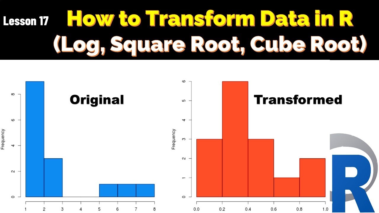
- YOUTUBE: Hướng dẫn chi tiết cách chuyển đổi dữ liệu trong R với các phương pháp log, căn bậc hai và căn bậc ba, giúp cải thiện phân tích dữ liệu.
Square Root Transformation in R
Square root transformation is a useful technique to stabilize variance and make the data more normal distribution-like. It is often used in the context of data analysis and statistical modeling. In R, you can apply a square root transformation using various methods.
Why Use Square Root Transformation?
- Stabilizes variance
- Reduces skewness
- Improves the normality of data
Applying Square Root Transformation
Here are some common ways to apply square root transformation in R:
Using the Base R
You can simply use the sqrt() function in R to transform your data. For example:
# Sample data
data <- c(1, 4, 9, 16, 25)

# Apply square root transformation
sqrt_data <- sqrt(data)

# Display the transformed data
print(sqrt_data)
Using dplyr for Data Frames
If you are working with data frames, the dplyr package provides a convenient way to apply transformations:
# Load dplyr package
library(dplyr)

# Sample data frame
df <- data.frame(value = c(1, 4, 9, 16, 25))

# Apply square root transformation
df <- df %>% mutate(sqrt_value = sqrt(value))

# Display the transformed data frame
print(df)
Using the caret Package for Preprocessing
The caret package can be used to preprocess data, including square root transformation:
# Load caret package
library(caret)

# Sample data frame
df <- data.frame(value = c(1, 4, 9, 16, 25))

# Define preprocessing method
preProcessParams <- preProcess(df, method = 'sqrt')

# Apply the transformation
transformed_df <- predict(preProcessParams, df)

# Display the transformed data frame
print(transformed_df)
Mathematical Explanation
The square root transformation is defined as:
where is the original data and is the transformed data.
Interpreting Results
After transformation, it is crucial to evaluate the results to ensure the transformation has the desired effect. Look at summary statistics, histograms, and normality tests to confirm improvements.
Conclusion
Square root transformation is a straightforward yet powerful tool in data preprocessing. Whether you're using base R, dplyr, or caret, transforming your data can help achieve better analytical results.
READ MORE:
Introduction to Square Root Transformation
Square root transformation is a statistical technique used to stabilize variance, reduce skewness, and make data more closely resemble a normal distribution. This method is particularly effective for data with a right-skewed distribution, where large values are disproportionately high.
The transformation is defined mathematically as:
where represents the original data values and represents the transformed data values. This transformation compresses the range of data, making the differences between small and large values less extreme.
Applying square root transformation in R can be done using several methods, such as:
- Using the
sqrt()function in base R - Applying the transformation within the
dplyrpackage - Preprocessing data with the
caretpackage
Here is a step-by-step approach to applying square root transformation in R:
- Load Your Data: Import your dataset into R using functions like
read.csv()orread.table(). - Inspect Your Data: Examine the structure and summary statistics of your data to understand its distribution and identify variables that may benefit from transformation.
- Apply the Transformation: Use the
sqrt()function to transform the relevant variables. For example, if your data is stored in a variable nameddata, you can transform it usingsqrt_data <- sqrt(data). - Verify the Transformation: Check the transformed data by plotting histograms, boxplots, or performing normality tests to ensure the transformation has the desired effect.
By understanding and applying square root transformation, you can improve the robustness of your statistical analyses and achieve more reliable results. This technique is especially useful in regression analysis, ANOVA, and other statistical modeling where homoscedasticity (equal variance) is a critical assumption.
Benefits of Square Root Transformation
Square root transformation is a powerful technique in data analysis, offering several key benefits for improving data quality and statistical analysis. Here are some of the primary benefits:
- Stabilizing Variance: By applying a square root transformation, the variance of the data is often stabilized. This is particularly useful for datasets with a high degree of variability.
- Reducing Skewness: Many datasets are right-skewed, with a long tail of higher values. The square root transformation compresses these high values, reducing skewness and making the data more symmetrical.
- Improving Normality: For statistical methods that assume normally distributed data, the square root transformation can help achieve a distribution that is closer to normal. This is important for accurate hypothesis testing and confidence interval estimation.
- Enhancing Linear Relationships: In regression analysis, the transformation can improve the linearity of relationships between variables, making models more accurate and interpretable.
- Mitigating the Impact of Outliers: Outliers can disproportionately influence the results of statistical analyses. The square root transformation reduces the impact of extreme values, leading to more robust and reliable results.
- Facilitating Data Interpretation: Transformed data can be easier to interpret, especially when dealing with counts or other non-negative variables. The transformation makes the range of values more manageable and comparable.
Mathematically, the transformation is defined as:
where represents the original data values and represents the transformed data values.
Here is a step-by-step approach to applying square root transformation and understanding its benefits:
- Identify Suitable Data: Determine which variables in your dataset would benefit from transformation, typically those with high variance or skewness.
- Apply the Transformation: Use the
sqrt()function in R to transform the selected variables. - Compare Distributions: Plot histograms or density plots of the original and transformed data to visualize changes in variance and skewness.
- Check Model Assumptions: In regression or ANOVA, re-evaluate the assumptions of normality and homoscedasticity to ensure they are better met with transformed data.
- Interpret Results: Analyze the statistical outputs with transformed data and compare them with those obtained from the original data to assess improvements in model performance and reliability.
By leveraging the benefits of square root transformation, analysts and researchers can enhance the quality of their data analyses, leading to more accurate and meaningful insights.
When to Use Square Root Transformation
Square root transformation is a valuable tool in data analysis, particularly effective under specific conditions. Here are some scenarios where using square root transformation can be beneficial:
- Right-Skewed Data: When your data is right-skewed, meaning it has a long tail of higher values, applying a square root transformation can help normalize the distribution and reduce skewness.
- Count Data: For count data, where values represent the number of occurrences of an event, the square root transformation can stabilize variance and make the data more normally distributed.
- Heteroscedasticity: If your data exhibits heteroscedasticity (non-constant variance), the square root transformation can help stabilize the variance, making it more homoscedastic (constant variance).
- Linear Regression: In linear regression models, if the residuals are not normally distributed or exhibit non-constant variance, transforming the dependent variable with a square root transformation can improve the model's assumptions and fit.
- Outlier Mitigation: When your dataset contains outliers that disproportionately affect your analysis, the square root transformation can reduce the impact of these extreme values, leading to more robust results.
- Biological Data: In biological and environmental sciences, measurements such as population sizes, concentrations, or other naturally occurring phenomena often benefit from square root transformation to meet statistical assumptions.
Here is a step-by-step guide on determining when to use square root transformation:
- Examine Data Distribution: Plot histograms or Q-Q plots to visually inspect the distribution of your data. Look for right-skewness or other deviations from normality.
- Check Variance: Analyze the variance of your data across different levels of the independent variables. Non-constant variance (heteroscedasticity) suggests the need for transformation.
- Evaluate Model Residuals: In regression analysis, examine residual plots. Non-normality or patterns in residuals may indicate the need for transforming the dependent variable.
- Apply Transformation: Use the
sqrt()function in R to apply the square root transformation to the relevant variables. - Reassess Distribution and Variance: After transformation, re-plot the histograms, Q-Q plots, and residuals to verify improvements in normality and homoscedasticity.
- Interpret Results: Analyze the transformed data and compare it to the original data to assess the effectiveness of the transformation. Check if the statistical assumptions are better met.
By following these steps, you can effectively determine when to use square root transformation and enhance the reliability and validity of your statistical analyses.
How to Apply Square Root Transformation in R
Applying a square root transformation in R is straightforward and can be done using various methods depending on the structure of your data and the specific requirements of your analysis. Below are step-by-step instructions on how to apply this transformation using different approaches:
Using Base R
The simplest way to apply a square root transformation is using the sqrt() function in base R. Here's how:
- Load Your Data: First, load your data into R. For example, if you have a vector of data:
- Apply the Square Root Transformation: Use the
sqrt()function to transform the data: - Verify the Transformation: Check the transformed data to ensure it has been applied correctly:
data <- c(1, 4, 9, 16, 25)sqrt_data <- sqrt(data)print(sqrt_data)Using dplyr for Data Frames
If you are working with data frames, the dplyr package provides a convenient way to apply the square root transformation:
- Load the dplyr Package: Ensure you have the
dplyrpackage installed and loaded: - Create a Data Frame: Create a sample data frame:
- Apply the Transformation: Use the
mutate()function to apply the square root transformation: - Verify the Transformation: Check the transformed data frame:
install.packages("dplyr")
library(dplyr)df <- data.frame(value = c(1, 4, 9, 16, 25))df <- df %>% mutate(sqrt_value = sqrt(value))print(df)Using caret Package for Preprocessing
The caret package is useful for preprocessing data, including applying transformations:
- Load the caret Package: Ensure you have the
caretpackage installed and loaded: - Create a Data Frame: Create a sample data frame:
- Define Preprocessing Method: Specify the preprocessing method:
- Apply the Transformation: Use the
predict()function to transform the data: - Verify the Transformation: Check the transformed data frame:
install.packages("caret")
library(caret)df <- data.frame(value = c(1, 4, 9, 16, 25))preProcessParams <- preProcess(df, method = 'sqrt')transformed_df <- predict(preProcessParams, df)print(transformed_df)By following these methods, you can effectively apply square root transformation in R, improving the quality of your data and the robustness of your statistical analyses.
Square Root Transformation Using Base R
Applying a square root transformation using Base R is straightforward and involves simple, intuitive steps. This transformation is beneficial for stabilizing variance, reducing skewness, and making data more normally distributed. Below is a detailed guide on how to perform a square root transformation using Base R:
- Load Your Data: First, you need to load your data into R. You can create a vector or import data from a file. For example, to create a sample vector of data:
- Apply the Square Root Transformation: Use the
sqrt()function to transform the data. This function computes the square root of each element in the vector: - Verify the Transformation: Print the transformed data to ensure the transformation has been applied correctly:
- Plotting the Data: To visually compare the original and transformed data, you can create plots. For example, using the
plot()function: - Applying to Data Frames: If your data is in a data frame, you can apply the transformation to a specific column. For example, consider a data frame
df: - Verify the Data Frame Transformation: Print the data frame to check the new column with the transformed values:
data <- c(1, 4, 9, 16, 25)sqrt_data <- sqrt(data)print(sqrt_data)The output will be:
[1] 1 2 3 4 5par(mfrow = c(1, 2)) # Set up the plotting area
plot(data, main = "Original Data", xlab = "Index", ylab = "Value", type = "b")
plot(sqrt_data, main = "Square Root Transformed Data", xlab = "Index", ylab = "Value", type = "b")This code will generate side-by-side plots of the original and transformed data, allowing you to visually assess the effects of the transformation.
df <- data.frame(value = c(1, 4, 9, 16, 25))
df$sqrt_value <- sqrt(df$value)print(df)The output will be:
  value sqrt_value
1     1          1
2     4          2
3     9          3
4    16          4
5    25          5
By following these steps, you can effectively apply square root transformation to your data using Base R. This simple yet powerful technique helps improve the quality and interpretability of your statistical analyses.
Square Root Transformation with dplyr Package
The dplyr package in R provides a powerful and easy-to-use set of tools for data manipulation, including the application of transformations like the square root transformation. Here is a step-by-step guide on how to use dplyr for this purpose:
- Install and Load the dplyr Package: If you haven't already installed
dplyr, you can do so using the following command: - Create or Load a Data Frame: Create a sample data frame or load your existing data. For example:
- Apply the Square Root Transformation: Use the
mutate()function fromdplyrto add a new column with the square root transformed values: - Verify the Transformation: Print the data frame to check the new column with the transformed values:
- Chain Multiple Transformations: You can chain multiple transformations and operations using the pipe operator
%>%. For example, if you want to filter the data and then apply the transformation: - Plotting the Data: To visualize the original and transformed data, you can use the
ggplot2package. Install and loadggplot2if you haven't already:
install.packages("dplyr")Then, load the package into your R session:
library(dplyr)df <- data.frame(value = c(1, 4, 9, 16, 25))df <- df %>%
mutate(sqrt_value = sqrt(value))print(df)The output will be:
  value sqrt_value
1     1          1
2     4          2
3     9          3
4    16          4
5 25 5df <- df %>%
filter(value > 2) %>%
mutate(sqrt_value = sqrt(value))install.packages("ggplot2")
library(ggplot2)Create plots to compare the original and transformed data:
ggplot(df, aes(x = value, y = sqrt_value)) +
  geom_point() +
  geom_line() +
  ggtitle("Square Root Transformation with dplyr") +
  xlab("Original Value") +
  ylab("Square Root Transformed Value")
By following these steps, you can efficiently apply square root transformations to your data using the dplyr package, enhancing your data manipulation capabilities in R.
Applying Square Root Transformation in Data Frames
Applying a square root transformation to data frames in R is a common practice to stabilize variance and make data more normally distributed. This process can be done easily using both Base R and packages like dplyr. Below is a step-by-step guide on how to apply square root transformation in data frames:
- Load Your Data: First, load your data into a data frame. You can create a sample data frame or load data from a file. For example:
- Using Base R: Apply the square root transformation directly to a column in the data frame using Base R functions.
- Using dplyr: The
dplyrpackage provides a more readable and efficient way to manipulate data frames. Ensure you have thedplyrpackage installed and loaded: - Apply the Transformation with dplyr: Use the
mutate()function to add a new column with the transformed values: - Verify the Transformation: Print the data frame to ensure the transformation has been applied correctly:
- Multiple Transformations and Operations: You can chain multiple operations using the pipe operator
%>%. For example, you can filter the data and then apply the transformation: - Plotting the Data: To visualize the effects of the transformation, use the
ggplot2package. Install and loadggplot2if you haven't already:
df <- data.frame(value = c(1, 4, 9, 16, 25))df$sqrt_value <- sqrt(df$value)This will create a new column in the data frame with the square root transformed values.
install.packages("dplyr")
library(dplyr)df <- df %>%
mutate(sqrt_value = sqrt(value))print(df)The output will be:
  value sqrt_value
1     1          1
2     4          2
3     9          3
4    16          4
5 25 5df <- df %>%
filter(value > 2) %>%
mutate(sqrt_value = sqrt(value))install.packages("ggplot2")
library(ggplot2)Create plots to compare the original and transformed data:
ggplot(df, aes(x = value, y = sqrt_value)) +
  geom_point() +
  geom_line() +
  ggtitle("Square Root Transformation in Data Frames") +
  xlab("Original Value") +
  ylab("Square Root Transformed Value")
By following these steps, you can effectively apply square root transformation to data frames in R, enhancing your data analysis process.
Preprocessing Data with caret Package
The caret package in R is a powerful tool for pre-processing data before model training. It provides various methods to prepare your data, ensuring it meets the requirements for robust statistical analysis and machine learning models. Below are the steps and methods you can use for preprocessing data with the caret package:
-
Loading the caret package:
library(caret) -
Loading the dataset:
data(iris) summary(iris[,1:4]) -
Applying transformations:
-
Centering: Subtracts the mean from each feature.
preprocessParams <- preProcess(iris[,1:4], method=c("center")) transformed <- predict(preprocessParams, iris[,1:4]) summary(transformed) -
Scaling: Divides each feature by its standard deviation.
preprocessParams <- preProcess(iris[,1:4], method=c("scale")) transformed <- predict(preprocessParams, iris[,1:4]) summary(transformed) -
Standardizing: Centers and scales the data.
preprocessParams <- preProcess(iris[,1:4], method=c("center", "scale")) transformed <- predict(preprocessParams, iris[,1:4]) summary(transformed) -
Square Root Transformation: Applies square root transformation to reduce skewness.
preprocessParams <- preProcess(iris[,1:4], method=c("BoxCox"))
transformed <- predict(preprocessParams, iris[,1:4])
summary(transformed)
-
-
Handling missing values:
- K-Nearest Neighbors: Imputes missing values based on the nearest neighbors.
- Bagged Trees: Uses a bagged tree model to predict and impute missing values.
- Median Imputation: Replaces missing values with the median of the column.
preprocessParams <- preProcess(iris[,1:4], method=c("knnImpute"))
transformed <- predict(preprocessParams, iris[,1:4])
summary(transformed)
Using these preprocessing steps, you can ensure that your data is clean, normalized, and ready for any further analysis or machine learning tasks. The caret package simplifies these processes, making it easier to handle complex datasets with various preprocessing requirements.
Examples of Square Root Transformation in R
The square root transformation is a useful technique to stabilize variance and make the data more normally distributed. Below are examples demonstrating how to apply this transformation in R.
Example 1: Basic Square Root Transformation
To apply a square root transformation to a simple numeric vector:
# Define a numeric vector
x <- c(1, 4, 9, 16, 25)

# Apply square root transformation
sqrt_x <- sqrt(x)

# Print the transformed values
print(sqrt_x)
The resulting output will be:
[1] 1 2 3 4 5
Example 2: Handling Negative Values
When your data contains negative values, you should take the absolute value before applying the square root transformation to avoid NaNs:
# Define a vector with negative values
x <- c(1, -4, 9, -16, 25)

# Apply square root transformation to absolute values
sqrt_x <- sqrt(abs(x))

# Print the transformed values
print(sqrt_x)
The resulting output will be:
[1] 1.000000 2.000000 3.000000 4.000000 5.000000
Example 3: Square Root Transformation on Data Frame Columns
To apply the square root transformation to specific columns in a data frame:
# Create a data frame
data <- data.frame(
  a = c(1, 3, 4, 6, 8, 9),
  b = c(7, 8, 8, 7, 13, 16),
  c = c(11, 13, 13, 18, 19, 22)
)

# Apply square root transformation to column 'a'
data$a_sqrt <- sqrt(data$a)

# Print the transformed data frame
print(data)
The resulting output will be:
  a  b  c   a_sqrt
1 1  7 11 1.000000
2 3  8 13 1.732051
3 4  8 13 2.000000
4 6  7 18 2.449490
5 8 13 19 2.828427
6 9 16 22 3.000000
Example 4: Square Root Transformation Using the dplyr Package
Using dplyr to apply a square root transformation to multiple columns:
# Load dplyr package
library(dplyr)

# Apply square root transformation to multiple columns
data_transformed <- data %>%
  mutate(across(c(a, b), sqrt))

# Print the transformed data frame
print(data_transformed)
The resulting output will be:
        a        b  c
1 1.000000 2.645751 11
2 1.732051 2.828427 13
3 2.000000 2.828427 13
4 2.449490 2.645751 18
5 2.828427 3.605551 19
6 3.000000 4.000000 22
Example 5: Square Root Transformation Using the recipes Package
Applying square root transformation within a preprocessing pipeline using the recipes package:
# Load the required packages
library(recipes)
library(dplyr)

# Create a recipe
rec <- recipe(~ ., data = data) %>%
  step_sqrt(all_numeric_predictors())

# Prepare the recipe
rec_prep <- prep(rec, training = data)

# Apply the transformation
data_transformed <- bake(rec_prep, new_data = data)

# Print the transformed data frame
print(data_transformed)
The resulting output will be:
        a        b  c
1 1.000000 2.645751 11
2 1.732051 2.828427 13
3 2.000000 2.828427 13
4 2.449490 2.645751 18
5 2.828427 3.605551 19
6 3.000000 4.000000 22
By following these examples, you can efficiently apply square root transformations to your data in R, improving the normality of the distributions and stabilizing variances.
Mathematical Explanation of Square Root Transformation
The square root transformation is a commonly used technique in statistics to normalize data and stabilize variance. This transformation is especially useful for data that follows a Poisson distribution or exhibits right skewness. The mathematical basis for this transformation is rooted in the power transformations family, specifically as a special case of the Box-Cox transformation with \(\lambda = 0.5\).
Mathematically, the square root transformation can be expressed as:
or , where \(y\) is the original variable.
Here's how the transformation works:
- Normalization of Data: When a dataset has a right-skewed distribution, applying the square root transformation helps to make the distribution more symmetrical. This is particularly useful for meeting the assumptions of parametric tests, which require normally distributed data.
- Variance Stabilization: For data with heteroscedasticity (non-constant variance), the square root transformation can stabilize the variance, making the data more suitable for regression models and other statistical analyses.
Let's look at an example to illustrate the effect of the square root transformation:
Suppose we have a dataset with a variable \(y\) representing count data (e.g., number of occurrences of an event). The original data may look like this:
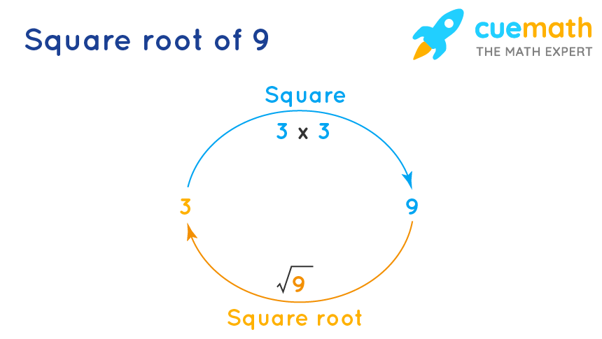
| Original Data (\(y\)) | Transformed Data (\(\sqrt{y}\)) |
|---|---|
| 1 | 1 |
| 4 | 2 |
| 9 | 3 |
| 16 | 4 |
| 25 | 5 |
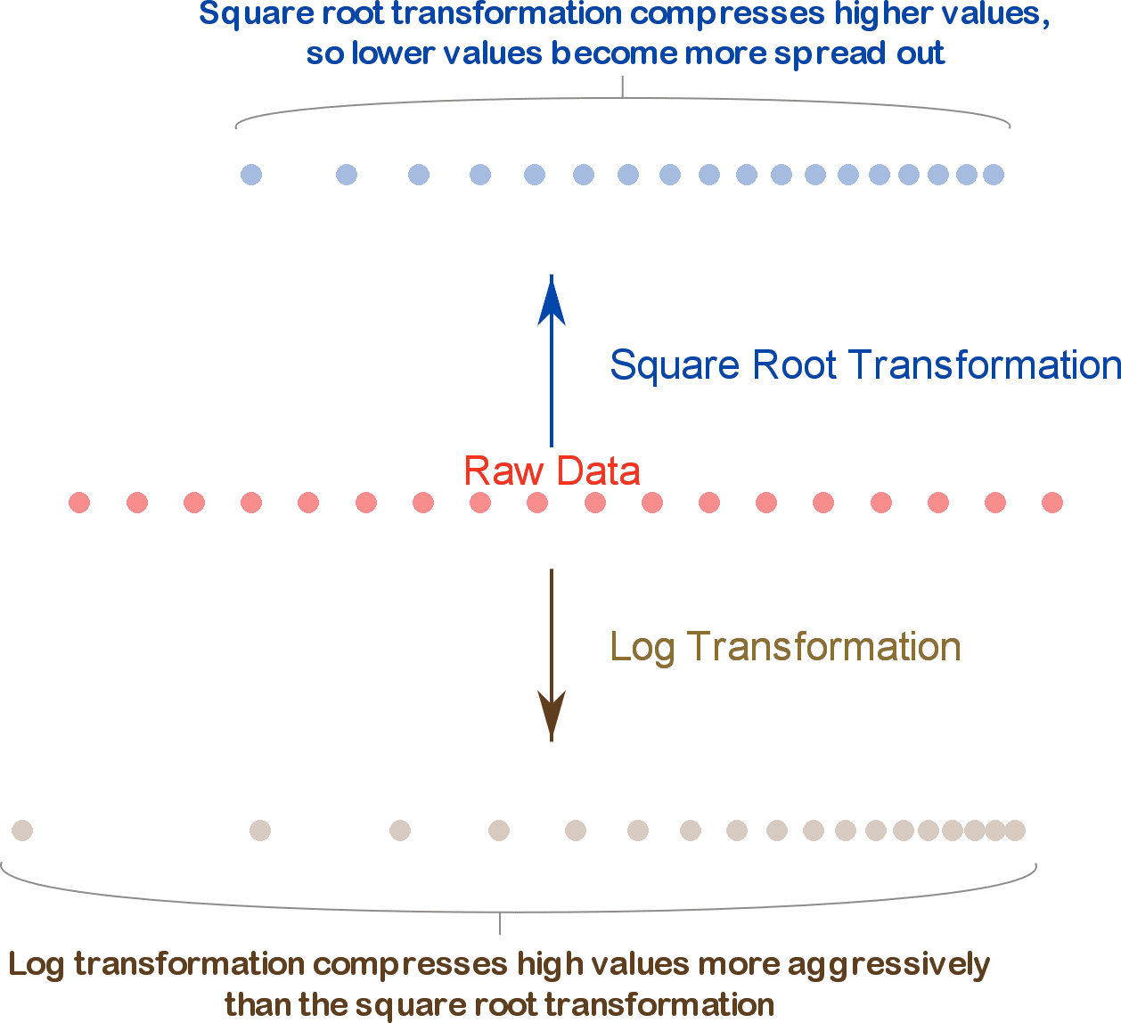
After transformation, the high values are compressed, and the lower values are more spread out. This helps in reducing skewness and making the data more normally distributed. The transformed data is now more suitable for linear regression and other analyses that assume normality.
The transformation also helps in reducing the impact of outliers by compressing the scale of the data. However, one must be cautious when applying this transformation to data with negative values, as the square root of a negative number is not defined in the real number system.
In summary, the square root transformation is a powerful tool for normalizing skewed data and stabilizing variance, thus improving the performance and validity of various statistical analyses.
Interpreting Results After Transformation
After applying a square root transformation to your data, it is crucial to understand how to interpret the transformed results correctly. Here are some key points to guide you through this process:
-
Understanding the Transformation Impact:
The square root transformation is typically used to stabilize variance and reduce skewness in your data. This can make the data more suitable for linear modeling and improve the validity of statistical tests. However, it also means that the interpretation of results will differ from those of the original data.
-
Interpreting Transformed Values:
When you analyze the transformed data, remember that the results are on the square root scale. For instance, if you have applied the transformation to a variable \(y\), then the new variable is \(\sqrt{y}\). To make meaningful inferences about the original data, you might need to back-transform the results.
-
Back-Transformation:
To interpret results in the original scale, square the values obtained from the analysis. For example, if a transformed mean is 3, the mean in the original scale would be \(3^2 = 9\). However, note that variances and other summary statistics may not back-transform as straightforwardly.
-
Effect on Statistical Tests:
After transformation, the p-values and significance levels may change. It's essential to assess whether the transformed model meets the assumptions of the statistical tests being used. Often, the transformation helps in achieving homoscedasticity and normality, thus providing more reliable test results.
-
Comparing Models:
Comparing models before and after transformation can highlight the transformation's effect. For instance, if an interaction term was significant before transformation but not after, it may indicate that the original model's assumptions were violated, leading to spurious findings.
-
Interpreting Coefficients:
Coefficients from regression models fitted to transformed data represent the effect on the transformed outcome. To interpret these in the context of the original data, consider how changes in predictor variables influence the square root of the outcome. For example, if the coefficient for a predictor is 2 in the transformed model, it means a one-unit increase in the predictor results in an average increase of 2 in the square root of the outcome.
Interpreting results after a square root transformation requires careful consideration of the transformation's impact on data distribution, statistical assumptions, and the interpretability of findings. By following these guidelines, you can make meaningful and accurate inferences from your transformed data.
Common Mistakes to Avoid
Applying square root transformation in R can significantly improve the analysis, but it is essential to be aware of common mistakes to avoid:
- Ignoring Negative Values:
The square root transformation cannot be applied to negative values directly. Applying it to datasets with negative values will result in errors or missing values. Ensure all values are non-negative or shift the data by adding a constant before applying the transformation.
- Misinterpreting Transformed Data:
After transformation, the scale and distribution of data change. Ensure you interpret the results correctly in the context of the transformed scale. For instance, means and standard deviations will no longer be on the original scale, affecting the interpretation of summary statistics.
- Overlooking Assumptions of Normality:
One of the primary reasons for applying square root transformation is to normalize data. However, not all data distributions benefit from this transformation. Verify the normality of the data post-transformation using Q-Q plots or other diagnostic tools.
- Failing to Check for Heteroscedasticity:
Square root transformation helps in stabilizing variance (homoscedasticity). Always check residual plots after transformation to ensure that the variance of residuals is consistent across fitted values.
- Using Inappropriate Transformation for Left-Skewed Data:
Square root transformation is generally effective for right-skewed data. Applying it to left-skewed data can exacerbate the skewness. For left-skewed data, consider other transformations like log or cube root.
- Inconsistent Application:
Consistency is crucial when applying transformations. Ensure the same transformation is applied across all relevant parts of the analysis, including during data preprocessing, model fitting, and result interpretation.
- Neglecting Model Interpretability:
While transformations can improve statistical properties of the data, they can also make the model coefficients less interpretable. Always consider the trade-off between statistical correctness and interpretability.
By avoiding these common mistakes, you can effectively utilize square root transformation to improve the robustness and reliability of your statistical analyses in R.

Advantages and Disadvantages
The square root transformation is a valuable tool in data analysis, offering several advantages and disadvantages. Here is a detailed breakdown:
Advantages
- Reduces Skewness: Square root transformation is effective in reducing right-skewness in the data, making it closer to a normal distribution. This can improve the performance of statistical models that assume normality.
- Handles Zero Values: Unlike logarithmic transformations, square root transformations can be applied to data that includes zero values, making it more versatile in certain datasets.
- Preserves Relationships: This transformation tends to preserve the original relationships in the data, which is beneficial when analyzing correlations and trends.
- Simpler Interpretation: The results of a square root transformation are often easier to interpret compared to more complex transformations like Box-Cox.
Disadvantages
- Limited Effect on Strongly Skewed Data: For data that is highly skewed, square root transformation may not be strong enough to achieve normality. In such cases, stronger transformations like logarithmic or Box-Cox might be needed.
- Less Effective for Negative Values: Since the square root of a negative number is not defined in the real number system, this transformation cannot be directly applied to datasets with negative values.
- Reduction in Variability: While it reduces skewness, it also reduces the variability in the data, which may not be desirable in all analyses.
- Potential Misinterpretation: If not properly understood, the transformed values can be misinterpreted, especially by those unfamiliar with the transformation process.
Understanding these advantages and disadvantages helps in making an informed decision about when to use square root transformation in R, ensuring it aligns with the goals of the data analysis.
Comparing Square Root Transformation with Other Transformations
Square root transformation is one of several methods used to transform data to meet the assumptions of statistical analyses or to make data more interpretable. Here, we compare square root transformation with other common transformation techniques such as logarithmic, cube root, and power transformations.
1. Square Root Transformation
The square root transformation is particularly useful for data with moderate skewness. It stabilizes variance and makes the data distribution more normal. The transformation is defined as:
\[ Y' = \sqrt{Y} \]
This method reduces the relative impact of large values but is less aggressive than logarithmic transformation.
2. Logarithmic Transformation
Logarithmic transformation is often used for highly skewed data. It compresses the range of the data and can handle large differences in magnitude. The transformation is defined as:
\[ Y' = \log(Y) \]
It's especially effective when the data spans several orders of magnitude. However, it cannot be applied to zero or negative values unless a constant is added.
3. Cube Root Transformation
Cube root transformation is another alternative for dealing with skewed data. It is defined as:
\[ Y' = \sqrt[3]{Y} \]
This transformation is less drastic than the logarithmic transformation and is useful when the data contains negative values since the cube root of negative numbers is defined.
4. Power Transformation
Power transformations include a family of transformations, such as the Box-Cox transformation, that raise the data to a power. This method can be tailored to the data by choosing an appropriate power (lambda). The general form is:
\[ Y' = Y^\lambda \]
Depending on the chosen lambda, this transformation can approximate both square root and logarithmic transformations, offering flexibility in achieving normality and variance stabilization.
5. Comparison and Use Cases
- Square Root Transformation: Ideal for count data and moderately skewed distributions.
- Logarithmic Transformation: Suitable for highly skewed data, particularly when dealing with multiplicative processes or data that spans several orders of magnitude.
- Cube Root Transformation: Useful for data that includes negative values and is moderately skewed.
- Power Transformation: Versatile, can be tuned to the specific needs of the data, useful for achieving normality and homoscedasticity.
Each transformation has its strengths and is suited to different types of data and analysis goals. Choosing the right transformation depends on the specific characteristics of the data and the assumptions underlying the statistical methods being used.
Conclusion and Best Practices
Applying a square root transformation in R can significantly enhance the quality of your data analysis, particularly when dealing with skewed distributions or heteroscedasticity. Here are some key takeaways and best practices for using this technique effectively:
Conclusion
The square root transformation is a valuable tool in data preprocessing. By compressing high values and spreading out low values, it helps to stabilize variance and make patterns in the data more apparent. This transformation is particularly useful for right-skewed data and can improve the performance of parametric statistical tests and regression models.
Best Practices
- Check for Skewness: Always inspect your data for skewness before applying the square root transformation. Use visualizations like histograms and statistical measures such as skewness coefficient.
- Pre-Processing Steps: Clean your data to handle missing values and outliers. Ensure that all values are non-negative, as the square root of negative numbers is not defined in real numbers.
- Apply Transformation Appropriately: Use the transformation only when necessary. Overuse can lead to overfitting and may obscure the interpretability of your results.
- Compare with Other Transformations: Evaluate the performance of the square root transformation against other transformations like log or Box-Cox to determine the best fit for your data.
- Document Transformations: Keep a detailed record of all transformations applied to your data. This is crucial for reproducibility and for explaining your methodology in reports or publications.
- Analyze Residuals: After applying the transformation, check the residuals of your regression models to ensure that the assumptions of normality and homoscedasticity are met.
- Use with Caution in Visualizations: When creating visualizations, clearly indicate if a transformation has been applied to avoid misleading interpretations.
By following these best practices, you can effectively leverage square root transformation to enhance your data analysis in R, ensuring more reliable and interpretable results.
Further Reading and Resources
For those interested in diving deeper into the concept and application of square root transformation in R, the following resources provide valuable insights and examples:
- Quantifying Health - This website offers a comprehensive beginner's guide to square root transformation, including its application in normalizing skewed distributions, transforming non-linear relationships, reducing heteroscedasticity, and improving visualization clarity. It also discusses the limitations and appropriate contexts for using square root transformations.
- Statology - Statology provides practical examples of how to apply the square root transformation to vectors and data frames in R. It explains the syntax and includes sample code, making it an excellent resource for those looking to implement these transformations in their own data analysis projects.
- R-bloggers - This blog aggregates posts from various R users and experts, often featuring tutorials and case studies on data transformations, including the square root transformation. It’s a good place to find community-driven content and real-world applications.
- Books on Data Analysis and Regression Models - Many textbooks on statistical analysis and regression modeling cover the theory and application of data transformations, including the square root transformation. Titles such as "Data Analysis Using Regression and Multilevel/Hierarchical Models" are particularly recommended for their in-depth treatment of these topics.
- Online Courses and Tutorials - Platforms like Coursera, edX, and Udemy offer courses on R programming and data analysis that include sections on data transformations. These can provide structured learning paths with video lectures, hands-on exercises, and peer support.
- Research Articles and Journals - For those interested in the theoretical underpinnings and advanced applications of square root transformations, academic journals and research articles are invaluable. Sites like JSTOR and Google Scholar can help locate these resources.
These resources offer a mix of theoretical knowledge, practical examples, and community insights, helping both beginners and advanced users effectively apply square root transformations in R.

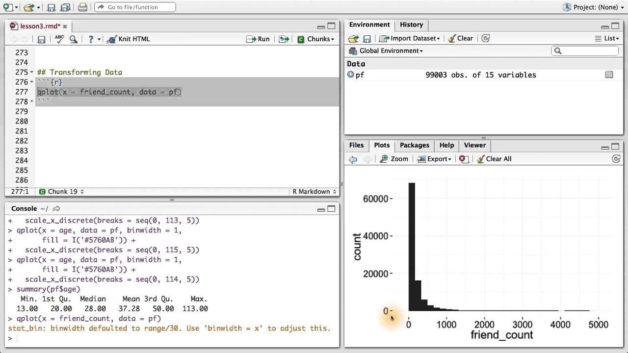
Hướng dẫn chi tiết cách chuyển đổi dữ liệu trong R với các phương pháp log, căn bậc hai và căn bậc ba, giúp cải thiện phân tích dữ liệu.
Cách Chuyển Đổi Dữ Liệu Trong R | Log, Căn Bậc Hai, Căn Bậc Ba Trong R
READ MORE:
Hướng dẫn sử dụng phép biến đổi căn bậc hai để cải thiện mô hình tuyến tính trong R. Video này giúp bạn hiểu rõ hơn về cách sử dụng R để thực hiện phép biến đổi này và tối ưu hóa kết quả phân tích dữ liệu của bạn.
Sử dụng phép biến đổi căn bậc hai để cải thiện mô hình tuyến tính