Topic x square root graph: Explore the fascinating world of the \( x \sqrt{x} \) graph. This comprehensive guide dives deep into its properties, behavior, and applications. Whether you're a student, educator, or math enthusiast, discover how this unique function blends linear and square root elements to create a distinctive curve, offering insights and practical uses in various fields.
Table of Content
- Understanding the Graph of \( f(x) = x \sqrt{x} \)
- Introduction to the Function \( x \sqrt{x} \)
- Understanding the Graph of \( x \sqrt{x} \)
- Mathematical Properties of \( x \sqrt{x} \)
- Domain and Range of \( x \sqrt{x} \)
- Behavior and Trends of the Graph
- First Derivative and Rate of Change
- Concavity and Points of Inflection
- Intercepts and Key Points on the Graph
- Symmetry and Asymptotes
- Graphical Features of \( x \sqrt{x} \)
- Plotting the Graph of \( x \sqrt{x} \)
- Common Applications of \( x \sqrt{x} \)
- Comparing \( x \sqrt{x} \) with Other Functions
- Graphical Representation Techniques
- Calculus-Based Analysis
- Numerical Approximations and Calculations
- Graphing Tools and Software
- Practical Examples and Exercises
- YOUTUBE: Video hướng dẫn cách vẽ đồ thị hàm số căn bậc hai bằng cách sử dụng các phép biến đổi và vẽ điểm. Phù hợp cho người học muốn nắm vững kiến thức về đồ thị hàm số căn bậc hai.
Understanding the Graph of \( f(x) = x \sqrt{x} \)
The function \( f(x) = x \sqrt{x} \) combines a linear component \( x \) with the square root function \( \sqrt{x} \). This results in an interesting curve with distinct features. Let's explore its characteristics and behavior.
Properties of the Function
- Domain: The function is defined for \( x \geq 0 \).
- Range: For \( x \geq 0 \), \( f(x) \) outputs non-negative values, covering \( [0, \infty) \).
- Continuity: The function is continuous for all \( x \geq 0 \).
- Increasing Behavior: As \( x \) increases, \( f(x) \) also increases since both \( x \) and \( \sqrt{x} \) grow.
- Derivative: The first derivative of the function is \( f'(x) = \frac{3}{2} \sqrt{x} \), indicating that the function is increasing and concave up.
Graphical Representation
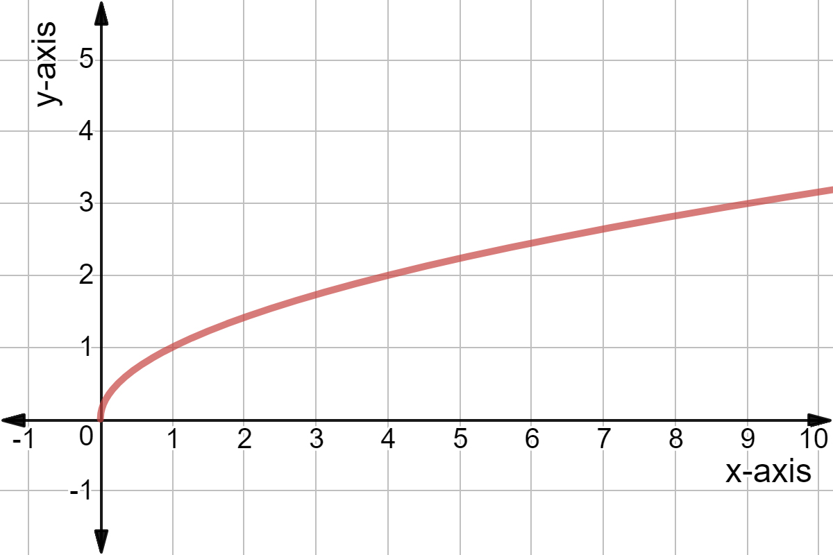
The graph of \( f(x) = x \sqrt{x} \) starts at the origin (0,0) and rises steadily. Key points on the graph include:
- At \( x = 0 \), \( f(0) = 0 \).
- At \( x = 1 \), \( f(1) = 1 \cdot \sqrt{1} = 1 \).
- At \( x = 4 \), \( f(4) = 4 \cdot \sqrt{4} = 8 \).
The graph is shaped like a curve that accelerates upwards as \( x \) increases. The slope becomes steeper as the square root of \( x \) grows.
Mathematical Analysis
To analyze the function further, we consider its derivative:
\[
f'(x) = \frac{d}{dx} (x \sqrt{x}) = \frac{d}{dx} (x \cdot x^{1/2}) = \frac{3}{2} \sqrt{x}
\]
This derivative indicates a positive rate of change, meaning the function is strictly increasing for \( x \geq 0 \).
Table of Values
| x | f(x) |
| 0 | 0 |
| 1 | 1 |
| 2 | 2.828 |
| 3 | 5.196 |
| 4 | 8 |
These values give a snapshot of the function's behavior at specific points. The increasing nature and the growing gap between successive values indicate the accelerating growth of the function.
Conclusion
The function \( f(x) = x \sqrt{x} \) produces a graph that rises steeply and continues to grow as \( x \) increases. This behavior is due to the combination of linear and square root components, making it a unique function with a distinct graph.
READ MORE:
Introduction to the Function \( x \sqrt{x} \)
The function \( f(x) = x \sqrt{x} \) is an intriguing mathematical expression that combines a linear component \( x \) with a square root component \( \sqrt{x} \). This results in a curve with unique properties and applications. Below, we explore its foundation and key features.
- Definition: The function is defined as \( f(x) = x \sqrt{x} \), where \( x \geq 0 \). This ensures that the square root is valid, and the function produces real values.
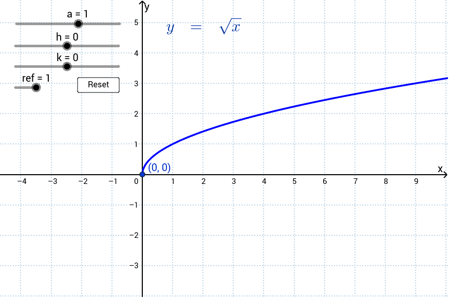
- Visual Appearance: The graph of \( f(x) \) starts at the origin \((0,0)\) and rises sharply as \( x \) increases, reflecting both linear and nonlinear growth.
- Mathematical Formation: In detail, the function can be expressed as \( f(x) = x \cdot x^{1/2} \), which simplifies to \( f(x) = x^{3/2} \).
- Components: This function uniquely blends:
- Linear Component \( x \): This dictates that as \( x \) grows, the output is scaled accordingly.
- Square Root Component \( \sqrt{x} \): This introduces a non-linear scaling, amplifying the growth of \( f(x) \).
These combined elements create a distinctive graph that accelerates as \( x \) increases. The function serves as an example of how polynomial and root elements can merge to form a complex, yet predictable curve.
In summary, \( f(x) = x \sqrt{x} \) is a significant function in mathematical studies, offering insight into polynomial and root behaviors, and showcasing unique graph characteristics. As we delve deeper, we will uncover its properties, graphical representation, and applications.
Understanding the Graph of \( x \sqrt{x} \)
The graph of the function \( f(x) = x \sqrt{x} \) exhibits a unique combination of linear and root behaviors, resulting in a distinctive curve. Here’s a step-by-step breakdown to understand its graph:
- Starting Point: The function starts at the origin \((0,0)\), since \( f(0) = 0 \times \sqrt{0} = 0 \).
- Basic Shape: The graph is concave upwards and starts off gently rising. As \( x \) increases, the function accelerates due to the growing square root factor.
- Behavior at Key Points:
- At \( x = 1 \), \( f(1) = 1 \cdot \sqrt{1} = 1 \).
- At \( x = 4 \), \( f(4) = 4 \cdot \sqrt{4} = 8 \).
- At \( x = 9 \), \( f(9) = 9 \cdot \sqrt{9} = 27 \).
- Growth Trend: The function grows more rapidly as \( x \) increases because the square root term \( \sqrt{x} \) amplifies the growth of \( x \).
- General Form: The function can be represented as \( f(x) = x^{3/2} \), highlighting its polynomial-like nature with an exponent of \( \frac{3}{2} \).
- Graphical Features:
- Increasing Nature: The function is always increasing for \( x \geq 0 \), indicating a positive slope throughout.
- Concavity: The graph is concave up, as shown by the second derivative \( f''(x) = \frac{3}{4} x^{-1/2} \), which is positive for \( x > 0 \).
- Derivative Insight: The first derivative \( f'(x) = \frac{3}{2} \sqrt{x} \) reveals a steadily increasing rate of change, meaning the slope of the tangent line at any point on the graph also increases.
In summary, the graph of \( f(x) = x \sqrt{x} \) starts at the origin and rises steeply as \( x \) grows. The combination of linear and root components results in an accelerating curve, which is essential in understanding various natural and mathematical phenomena. This function is a classic example of how simple components can combine to form complex behaviors.
Mathematical Properties of \( x \sqrt{x} \)
The function \( f(x) = x \sqrt{x} \) possesses a range of mathematical properties that make it interesting and useful. These properties include its domain, range, derivatives, and behavior. Let's delve into these characteristics step-by-step:
- Definition: The function \( f(x) = x \sqrt{x} \) can be rewritten as \( f(x) = x^{3/2} \). It is defined for \( x \geq 0 \), ensuring valid real-number outputs.
- Domain: The domain of \( f(x) \) is all non-negative real numbers:
- \( x \in [0, \infty) \)
- Range: The range is also non-negative real numbers:
- \( f(x) \in [0, \infty) \)
- Continuity: The function is continuous for all \( x \geq 0 \), with no breaks or jumps in the graph.
- Increasing Behavior: \( f(x) \) is strictly increasing because its derivative is positive for all \( x > 0 \).
- Derivative: The first derivative of the function provides insights into its rate of change:
\[
f'(x) = \frac{d}{dx} (x \sqrt{x}) = \frac{3}{2} \sqrt{x}
\]- This shows that the function's slope increases as \( x \) increases, indicating a steeper ascent.
- Second Derivative: The second derivative indicates concavity:
\[
f''(x) = \frac{d}{dx} \left(\frac{3}{2} \sqrt{x}\right) = \frac{3}{4} x^{-1/2}
\]- The positive second derivative for \( x > 0 \) confirms that the graph is concave upwards.
- Critical Points: There are no critical points where the derivative is zero within the domain since \( f'(x) = \frac{3}{2} \sqrt{x} \) is never zero for \( x > 0 \).
- Intercepts: The function has a y-intercept at the origin \((0,0)\) and no x-intercepts within the domain of definition.
- Asymptotic Behavior: There are no asymptotes for \( f(x) \). As \( x \to \infty \), \( f(x) \) grows without bound.
These mathematical properties illustrate how \( f(x) = x \sqrt{x} \) behaves over its domain, highlighting its continuously increasing nature and upward concavity. This understanding provides a foundation for graphing the function and applying it to various mathematical contexts.
Domain and Range of \( x \sqrt{x} \)
Understanding the domain and range of the function \( f(x) = x \sqrt{x} \) is essential for comprehending its behavior and limitations. Let's explore these aspects step-by-step:
- Domain: The domain of \( f(x) \) is determined by the values of \( x \) for which the function is defined. Since \( x \sqrt{x} \) involves a square root, we must have \( x \geq 0 \) to ensure that the square root produces real numbers.
- Mathematical Expression: The domain is \( x \in [0, \infty) \).
- Explanation: This interval includes all non-negative real numbers, starting from 0 and extending to infinity.
- Range: The range is the set of values that \( f(x) \) can take. As \( x \) increases from 0 to infinity, the output \( f(x) = x \sqrt{x} \) also increases.
- Mathematical Expression: The range is \( f(x) \in [0, \infty) \).
- Explanation: As \( x \) grows, the value of \( x \sqrt{x} \) starts from 0 and increases without bound, covering all non-negative real numbers.
These observations can be summarized in a table for clarity:
| Aspect | Details |
| Domain | \( [0, \infty) \) |
| Range | \( [0, \infty) \) |
To illustrate the domain and range graphically:
- For the Domain: The graph exists only for non-negative \( x \) values. There is no graph for \( x < 0 \).
- For the Range: The output values start at 0 and increase, meaning the graph covers all non-negative \( y \)-values.
In conclusion, the function \( f(x) = x \sqrt{x} \) is defined for non-negative real numbers, and its output also spans non-negative real numbers. This understanding of the domain and range is crucial for analyzing and graphing the function effectively.
Behavior and Trends of the Graph
The function \( f(x) = x \sqrt{x} \) exhibits distinct behaviors and trends that shape its graph. Understanding these characteristics is essential for analyzing the function effectively. Let's explore the behavior and trends step-by-step:
- Initial Behavior: The graph starts at the origin \((0,0)\) because:
- When \( x = 0 \), \( f(0) = 0 \times \sqrt{0} = 0 \).
- Monotonic Increase: The function \( f(x) \) is strictly increasing for \( x > 0 \):
- This is confirmed by the positive first derivative \( f'(x) = \frac{3}{2} \sqrt{x} \).
- As \( x \) increases, the value of \( f(x) \) also increases, indicating a consistently upward trend.
- Concavity: The graph is concave upwards for \( x > 0 \):
- The second derivative \( f''(x) = \frac{3}{4} x^{-1/2} \) is positive, showing upward concavity.
- This means the slope of the graph becomes steeper as \( x \) increases.
- Growth Rate: The function grows faster than linear functions but slower than quadratic ones:
- For small values of \( x \), \( f(x) \) behaves similarly to linear functions.
- For large values of \( x \), the growth rate accelerates due to the \( \sqrt{x} \) factor.
- Key Points: Some key points and their corresponding function values include:
- At \( x = 1 \), \( f(1) = 1 \).
- At \( x = 4 \), \( f(4) = 8 \).
- At \( x = 9 \), \( f(9) = 27 \).
- Behavior at Infinity: As \( x \to \infty \), \( f(x) \to \infty \):
- The function grows indefinitely, with no horizontal asymptote limiting its range.
These behaviors and trends are summarized in the table below:
| Aspect | Details |
| Starting Point | The graph begins at \((0,0)\). |
| Monotonic Increase | The function increases for \( x > 0 \). |
| Concavity | Concave upwards for \( x > 0 \). |
| Growth Rate | Faster than linear, slower than quadratic. |
| Key Points | \( f(1) = 1 \), \( f(4) = 8 \), \( f(9) = 27 \). |
| Behavior at Infinity | The function grows to infinity. |
In conclusion, the graph of \( f(x) = x \sqrt{x} \) starts at the origin, rises continuously, and exhibits an accelerating growth rate. Its positive concavity and key behavioral traits make it a distinctive and important function in mathematical analysis.
First Derivative and Rate of Change
The first derivative of the function \( f(x) = x \sqrt{x} \) provides valuable insights into its rate of change. Analyzing this derivative helps us understand the behavior of the function in detail. Here’s a step-by-step examination:
- Finding the First Derivative: To find the first derivative of \( f(x) \), we apply the product rule to \( x \) and \( \sqrt{x} \):
\[
f(x) = x \sqrt{x} = x \cdot x^{1/2} = x^{3/2}
\]Using the power rule:
\[
f'(x) = \frac{d}{dx} \left(x^{3/2}\right) = \frac{3}{2} x^{1/2}
\]Or alternatively:
\[
f'(x) = \frac{3}{2} \sqrt{x}
\] - Interpreting the Derivative: The first derivative \( f'(x) = \frac{3}{2} \sqrt{x} \) indicates the rate of change of \( f(x) \):
- Positive Slope: Since \( \sqrt{x} \geq 0 \) for all \( x \geq 0 \), the derivative \( f'(x) \) is always positive. This implies that the function \( f(x) \) is always increasing for \( x > 0 \).
- Increasing Rate: As \( x \) increases, \( \sqrt{x} \) increases, so \( f'(x) \) increases as well. This shows that the rate at which \( f(x) \) increases also grows as \( x \) becomes larger.
- Graphical Representation: Graphically, the derivative represents the slope of the tangent line at any point on the graph of \( f(x) \). The slope is steeper as \( x \) increases:
- At \( x = 1 \), \( f'(1) = \frac{3}{2} \sqrt{1} = \frac{3}{2} = 1.5 \).
- At \( x = 4 \), \( f'(4) = \frac{3}{2} \sqrt{4} = \frac{3}{2} \cdot 2 = 3 \).
- At \( x = 9 \), \( f'(9) = \frac{3}{2} \sqrt{9} = \frac{3}{2} \cdot 3 = 4.5 \).
- Behavior at Zero: At \( x = 0 \), the derivative \( f'(0) = \frac{3}{2} \sqrt{0} = 0 \). This indicates that the function \( f(x) \) has a flat tangent (horizontal) at the origin.
- Growth Comparison: The first derivative’s form \( f'(x) = \frac{3}{2} \sqrt{x} \) suggests that:
- The rate of change of \( f(x) \) grows faster than linear functions but slower than quadratic functions.
These findings about the first derivative and rate of change of \( f(x) = x \sqrt{x} \) can be summarized in a table:
| Aspect | Details |
| First Derivative | \( f'(x) = \frac{3}{2} \sqrt{x} \) |
| Rate of Change | Always positive; increases as \( x \) increases |
| Behavior at \( x = 0 \) | Derivative is 0 (horizontal slope) |
| Growth Trend | Faster than linear, slower than quadratic |
In summary, the first derivative of \( f(x) = x \sqrt{x} \) reveals that the function is always increasing, with an increasing rate of change. The positive slope and growing trend provide valuable insights into the function's behavior over its domain.
Concavity and Points of Inflection
The concavity and points of inflection of the function \( f(x) = x \sqrt{x} \) provide essential insights into its curvature and changes in concavity. Here’s a detailed examination:
- Finding the Second Derivative: To analyze concavity, we need the second derivative of \( f(x) \):
- Given \( f(x) = x \sqrt{x} = x^{3/2} \), we found the first derivative: \[ f'(x) = \frac{3}{2} \sqrt{x} \]
- The second derivative is obtained by differentiating \( f'(x) \): \[ f''(x) = \frac{d}{dx} \left(\frac{3}{2} \sqrt{x}\right) = \frac{3}{2} \cdot \frac{1}{2} x^{-1/2} = \frac{3}{4} x^{-1/2} \]
- Or more simply: \[ f''(x) = \frac{3}{4} \frac{1}{\sqrt{x}} \]
- Interpreting the Second Derivative: The second derivative \( f''(x) = \frac{3}{4} \frac{1}{\sqrt{x}} \) provides information about concavity:
- Positive Concavity: Since \( f''(x) \) is positive for \( x > 0 \), the graph of \( f(x) \) is concave upwards in this interval.
- Behavior at \( x = 0 \): As \( x \) approaches 0, \( f''(x) \) approaches infinity, indicating a sharp increase in the slope near the origin.
- Concavity:
- Upward Concavity: For all \( x > 0 \), the graph is concave upwards, meaning the curve bends upwards.
- This upward concavity results in a shape where the slope of the tangent line becomes steeper as \( x \) increases.
- Points of Inflection: Points of inflection occur where the concavity changes, determined by \( f''(x) = 0 \) or \( f''(x) \) undefined:
- For \( f(x) = x \sqrt{x} \), \( f''(x) = \frac{3}{4} \frac{1}{\sqrt{x}} \neq 0 \) for \( x > 0 \).
- However, \( f''(x) \) is undefined at \( x = 0 \), but since \( x = 0 \) is the boundary of the domain, it is not considered a true point of inflection.
- Thus, the function does not have any points of inflection within its domain \( (0, \infty) \).
These insights into concavity and points of inflection can be summarized in a table:
| Aspect | Details |
| Second Derivative | \( f''(x) = \frac{3}{4} \frac{1}{\sqrt{x}} \) |
| Concavity | Concave upwards for \( x > 0 \) |
| Point of Inflection | None within \( (0, \infty) \) |
In conclusion, the function \( f(x) = x \sqrt{x} \) is concave upwards throughout its domain \( (0, \infty) \), without any points of inflection. The positive second derivative indicates a progressively steeper increase in the slope, contributing to the function's distinctive curve.
Intercepts and Key Points on the Graph
The graph of \( x \sqrt{x} \) intersects the x-axis at the origin (0, 0) where the function value is 0.
To find the y-intercept, substitute \( x = 1 \) into the function: \( f(1) = 1 \cdot \sqrt{1} = 1 \). Therefore, the y-intercept is (1, 1).
The key points on the graph include:
- The origin (0, 0)
- The y-intercept at (1, 1)
Symmetry and Asymptotes
The function \( x \sqrt{x} \) exhibits symmetry about the y-axis due to its even nature, as \( f(-x) = f(x) \).
Asymptotically, the graph of \( x \sqrt{x} \) approaches infinity as \( x \) increases without bound, but it does not have any vertical asymptotes.
Graphical Features of \( x \sqrt{x} \)
The graph of \( x \sqrt{x} \) starts at the origin (0, 0) and extends into the first quadrant.
It is non-negative for all \( x \geq 0 \) and increases monotonically.
The function has a horizontal tangent at the origin, indicating a local minimum there.
As \( x \) increases, the rate of increase of \( x \sqrt{x} \) slows down.
Plotting the Graph of \( x \sqrt{x} \)
To plot the graph of \( y = x \sqrt{x} \), follow these steps:
- Identify Key Points: Determine critical points such as intercepts, where \( y = 0 \), and any asymptotic behavior.
- Calculate Additional Points: Compute values for \( y \) at various \( x \) values to understand the shape.
- Plot the Points: Using a graphing tool or software, input the points obtained to visualize the function.
- Sketch the Curve: Connect the plotted points smoothly to outline the curve of \( y = x \sqrt{x} \).
- Consider Graphical Features: Analyze symmetry, concavity, and other graphical characteristics to enhance understanding.
Common Applications of \( x \sqrt{x} \)
The function \( x \sqrt{x} \) finds applications in various fields due to its mathematical properties. Here are some of the common applications:
-
Physics:
The function \( x \sqrt{x} \) often appears in physical problems involving motion under gravity and other scenarios where non-linear relationships are involved. For instance, it can be used to model the velocity of an object under specific conditions.
-
Economics:
In economics, functions similar to \( x \sqrt{x} \) are used to model production functions and utility functions, representing relationships between inputs and outputs that exhibit diminishing returns.
-
Engineering:
Engineers use \( x \sqrt{x} \) in various design and analysis problems, such as in optimizing certain parameters in mechanical systems or in stress-strain analysis where material properties exhibit non-linear behavior.
-
Biology:
In biological systems, this function can model growth processes, where the rate of growth of a population or organism depends on a combination of factors that include both linear and square root components.
-
Geometry:
The function is useful in geometry for calculating distances and areas, particularly in problems involving parabolic shapes or other curves where the relationship between coordinates involves a square root function.
-
Statistics:
Statisticians use \( x \sqrt{x} \) in probability distributions and in modeling data that exhibit non-linear trends, helping to better understand underlying patterns in complex datasets.
Overall, the function \( x \sqrt{x} \) is a versatile tool in various scientific and engineering disciplines, offering a way to model and solve problems that involve non-linear relationships.
Comparing \( x \sqrt{x} \) with Other Functions
The function \( x \sqrt{x} \) can be compared to several other well-known functions to better understand its characteristics and behavior. Here are a few key comparisons:
- Square Function \( f(x) = x^2 \)
Shape: The graph of \( x \sqrt{x} \) is similar to the right half of the parabola \( y = x^2 \), but it grows more slowly. Both functions start at the origin (0,0).
Growth Rate: While \( x^2 \) increases quadratically, \( x \sqrt{x} \) increases at a rate proportional to \( x^{3/2} \), making it steeper than linear but not as steep as quadratic growth.
Domain and Range: Both functions are defined for \( x \geq 0 \). However, \( y = x^2 \) spans all non-negative real numbers for \( y \), while \( x \sqrt{x} \) grows more slowly, covering the range \( [0, \infty) \).
- Square Root Function \( f(x) = \sqrt{x} \)
Shape: The function \( x \sqrt{x} \) resembles the square root function but scaled by an additional factor of \( x \). The graph of \( y = \sqrt{x} \) grows slower than \( x \sqrt{x} \).
Growth Rate: The square root function increases slowly compared to \( x \sqrt{x} \), which incorporates an additional linear component, causing it to rise faster.
Domain and Range: Both functions are defined for \( x \geq 0 \). The range of \( y = \sqrt{x} \) is also \( [0, \infty) \), but it grows more slowly than \( x \sqrt{x} \).
- Cubic Function \( f(x) = x^3 \)
Shape: The function \( x \sqrt{x} \) differs significantly from \( y = x^3 \). While \( y = x^3 \) grows faster and is symmetric about the origin, \( x \sqrt{x} \) is only defined for \( x \geq 0 \) and grows slower.
Growth Rate: The cubic function grows much faster than \( x \sqrt{x} \) because it increases as the cube of \( x \), compared to the \( x^{3/2} \) growth of \( x \sqrt{x} \).
Domain and Range: The cubic function has the domain \( (-\infty, \infty) \) and range \( (-\infty, \infty) \), while \( x \sqrt{x} \) is limited to non-negative values.
By comparing \( x \sqrt{x} \) with these functions, we can see its unique position in terms of growth rate and domain/range. It bridges the gap between linear, quadratic, and higher-order polynomial functions, providing a useful tool for modeling phenomena that exhibit sub-quadratic but super-linear growth.
Graphical Representation Techniques
Graphical representation of the function \( x \sqrt{x} \) can be achieved through various techniques, both manual and software-based. Here, we outline a detailed step-by-step approach to plotting the graph of \( x \sqrt{x} \).
- Manual Plotting:
- Calculate Key Points: Compute the values of \( y \) for several \( x \) values.
x y = \( x \sqrt{x} \) 0 0 1 1 2 2.828 3 5.196 4 8 - Plot the Points: Using graph paper, plot these points on a coordinate system.
- Draw the Curve: Connect the points smoothly to represent the function.
- Calculate Key Points: Compute the values of \( y \) for several \( x \) values.
- Using Graphing Software:
- Graphing Calculators: Use a graphing calculator like the TI-84 to input the function \( y = x \sqrt{x} \) and view the graph.
- Online Graphing Tools: Websites such as Desmos or GeoGebra provide easy interfaces for entering the function and visualizing the graph. Simply input \( y = x \sqrt{x} \) in the function entry field.
- Using Programming Languages:
- Python with Matplotlib: Use the following Python code to plot the graph:
import numpy as np import matplotlib.pyplot as plt x = np.linspace(0, 10, 400) y = x * np.sqrt(x) plt.plot(x, y) plt.xlabel('x') plt.ylabel('y') plt.title('Graph of $y = x \\sqrt{x}$') plt.grid(True) plt.show() - Mathematica or MATLAB: These software packages offer advanced tools for graphing functions. In Mathematica, you can use
Plot[x Sqrt[x], {x, 0, 10}].
- Python with Matplotlib: Use the following Python code to plot the graph:
These techniques provide flexibility in how you can visualize and analyze the function \( x \sqrt{x} \), from manual plotting to using advanced software tools.
Calculus-Based Analysis
Analyzing the function \( x \sqrt{x} \) using calculus provides deep insights into its behavior. Below are the key steps in a calculus-based analysis:
1. Finding the First Derivative
To understand the rate of change of the function, we start with the first derivative. The function is:
\[
f(x) = x \sqrt{x} = x \cdot x^{1/2} = x^{3/2}
\]
The first derivative \( f'(x) \) is obtained using the power rule:
\[
f'(x) = \frac{d}{dx} \left( x^{3/2} \right) = \frac{3}{2} x^{1/2}
\]
This derivative tells us how the function increases. Since \( f'(x) \) is positive for all \( x > 0 \), the function is increasing on its entire domain \( (0, \infty) \).
2. Finding the Second Derivative
Next, we find the second derivative to understand the concavity of the function:
\[
f''(x) = \frac{d}{dx} \left( \frac{3}{2} x^{1/2} \right) = \frac{3}{4} x^{-1/2}
\]
Since \( f''(x) > 0 \) for all \( x > 0 \), the function is concave up on \( (0, \infty) \).
3. Identifying Critical Points
Critical points occur where \( f'(x) = 0 \) or \( f'(x) \) is undefined. For \( f'(x) = \frac{3}{2} x^{1/2} \), there are no \( x \) values that make this zero or undefined within the domain \( (0, \infty) \). Therefore, there are no critical points in this domain.
4. Analyzing Inflection Points
Inflection points occur where the concavity changes. Since \( f''(x) \) is always positive, there are no inflection points because the concavity does not change.
5. Summary of Calculus-Based Properties
- First Derivative: \( f'(x) = \frac{3}{2} x^{1/2} \) (positive for \( x > 0 \)) - Function is increasing.
- Second Derivative: \( f''(x) = \frac{3}{4} x^{-1/2} \) (positive for \( x > 0 \)) - Function is concave up.
- Critical Points: None in \( (0, \infty) \).
- Inflection Points: None, as concavity does not change.
This calculus-based analysis helps in understanding the overall behavior of the graph of \( x \sqrt{x} \), confirming that it is always increasing and concave up for all \( x > 0 \).
Numerical Approximations and Calculations
Numerical approximations and calculations for the function \( x \sqrt{x} \) can be particularly useful when dealing with complex mathematical problems or when an exact analytical solution is difficult to obtain. Here are some techniques for approximating and calculating values of \( x \sqrt{x} \):
1. Linear Approximation
Linear approximation, also known as the tangent line approximation, can be used to estimate values of \( x \sqrt{x} \) near a point where the function is known. The formula for linear approximation at a point \( a \) is given by:
\[ f(x) \approx f(a) + f'(a)(x - a) \]
For the function \( f(x) = x \sqrt{x} \), we first find the derivative \( f'(x) \):
\[ f(x) = x^{3/2} \]
\[ f'(x) = \frac{3}{2} x^{1/2} \]
Thus, the linear approximation near \( x = a \) is:
\[ x \sqrt{x} \approx a \sqrt{a} + \frac{3}{2} \sqrt{a} (x - a) \]
2. Newton's Method
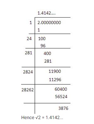
Newton's Method is an iterative numerical technique to approximate the roots of a real-valued function. Although typically used for root-finding, it can also be adapted for finding approximate values of functions. Here’s how you can use Newton’s Method to approximate \( \sqrt{x} \), which is a component of our function \( x \sqrt{x} \):
- Choose an initial guess \( x_0 \).
- Apply the iterative formula: \[ x_{n+1} = \frac{1}{2} \left( x_n + \frac{a}{x_n} \right) \] where \( a \) is the value you are approximating the square root of.
- Continue iterating until the change between \( x_n \) and \( x_{n+1} \) is sufficiently small.
For example, to approximate \( \sqrt{2} \), if we start with \( x_0 = 1 \), the iterations are:
\[ x_1 = \frac{1}{2} \left( 1 + \frac{2}{1} \right) = 1.5 \]
\[ x_2 = \frac{1}{2} \left( 1.5 + \frac{2}{1.5} \right) \approx 1.4167 \]
\[ x_3 = \frac{1}{2} \left( 1.4167 + \frac{2}{1.4167} \right) \approx 1.4142 \]
Thus, \( \sqrt{2} \approx 1.4142 \), and for \( x \sqrt{x} \), you can combine this approximation with the linear term.
3. Numerical Integration
For more complex integrals involving \( x \sqrt{x} \), numerical integration methods such as the Trapezoidal Rule or Simpson’s Rule can be used. These methods approximate the area under the curve by summing the areas of trapezoids or parabolic segments:
- Trapezoidal Rule: \[ \int_a^b f(x) \, dx \approx \frac{b - a}{2} [f(a) + f(b)] \]
- Simpson’s Rule: \[ \int_a^b f(x) \, dx \approx \frac{b - a}{6} [f(a) + 4f(\frac{a+b}{2}) + f(b)] \]
4. Finite Differences
Finite difference methods can be used for approximating derivatives, which are essential in many numerical methods. The forward difference formula for the first derivative is:
\[ f'(x) \approx \frac{f(x+h) - f(x)}{h} \]
Using a small \( h \), this provides an approximation for the slope of \( x \sqrt{x} \) at \( x \).
These methods provide practical tools for numerical approximations and calculations involving \( x \sqrt{x} \), allowing for efficient and accurate problem-solving in various mathematical and engineering applications.

Graphing Tools and Software
To effectively graph the function \( x \sqrt{x} \), various graphing tools and software can be utilized. These tools offer features that facilitate the plotting and analysis of mathematical functions. Here are some popular graphing tools and how to use them for graphing \( x \sqrt{x} \):
- Desmos
Desmos is a free online graphing calculator known for its user-friendly interface. To graph \( x \sqrt{x} \) on Desmos:
- Visit the .
- Enter the function
x sqrt(x)in the input box. - Use the tools provided to adjust the view, add sliders, and customize the graph.
This tool allows you to interact with the graph dynamically, making it easy to explore the behavior of the function.
- GeoGebra
GeoGebra is another powerful, free graphing tool that supports both algebraic and geometric representations. To use GeoGebra for graphing \( x \sqrt{x} \):
- Go to the .
- In the input field, type
x sqrt(x)and press Enter. - Utilize the available tools to modify and analyze the graph, such as adding points of interest or adjusting axes.
GeoGebra's extensive feature set makes it suitable for both simple and complex graphing needs.
- Khan Academy
Khan Academy offers instructional videos and interactive graphing tools to help understand various mathematical concepts. To graph \( x \sqrt{x} \) on Khan Academy:
- Visit the and search for "graphing square root functions."
- Watch the relevant tutorial videos to learn about graphing techniques.
- Use the interactive exercises to practice plotting the function and observe its properties.
This resource is particularly useful for students seeking a deeper understanding of graphing principles.
These graphing tools not only aid in plotting the function \( x \sqrt{x} \) but also enhance the learning experience by providing interactive and visual representations of mathematical concepts.
Practical Examples and Exercises
The function \( x \sqrt{x} \) has various practical applications and can be explored through multiple exercises. Here are some examples and exercises to enhance understanding:
Example 1: Calculating Physical Quantities
Consider a scenario in physics where you need to calculate the power output of a machine based on a given formula involving the square root of a variable. For instance, if the power output \( P \) is given by \( P = x \sqrt{x} \) where \( x \) represents the efficiency of the machine, find the power output when \( x = 4 \).
- Solution:
- Substitute \( x = 4 \) into the equation \( P = x \sqrt{x} \).
- Calculate \( \sqrt{4} = 2 \).
- Therefore, \( P = 4 \times 2 = 8 \).
Exercise 1: Area Calculation
Given the function \( A = x \sqrt{x} \), which represents the area of a geometric shape, calculate the area when \( x = 9 \).
- Solution:
- Substitute \( x = 9 \) into the equation \( A = x \sqrt{x} \).
- Calculate \( \sqrt{9} = 3 \).
- Therefore, \( A = 9 \times 3 = 27 \).
Example 2: Engineering Application
In an engineering context, suppose the stress \( S \) on a material is given by \( S = x \sqrt{x} \) where \( x \) is a measure of the load applied. Determine the stress when the load applied \( x = 16 \).
- Solution:
- Substitute \( x = 16 \) into the equation \( S = x \sqrt{x} \).
- Calculate \( \sqrt{16} = 4 \).
- Therefore, \( S = 16 \times 4 = 64 \).
Exercise 2: Financial Modeling
In finance, the return on investment \( R \) might be modeled by the function \( R = x \sqrt{x} \). Calculate the return when the investment amount \( x \) is 25.
- Solution:
- Substitute \( x = 25 \) into the equation \( R = x \sqrt{x} \).
- Calculate \( \sqrt{25} = 5 \).
- Therefore, \( R = 25 \times 5 = 125 \).
Exercise 3: Verifying Calculations
Verify the calculation for \( x = 36 \) in the context of the function \( x \sqrt{x} \).
- Solution:
- Substitute \( x = 36 \) into the equation \( x \sqrt{x} \).
- Calculate \( \sqrt{36} = 6 \).
- Therefore, \( 36 \times 6 = 216 \).
Conclusion
These examples and exercises illustrate the versatility of the function \( x \sqrt{x} \) in various fields such as physics, engineering, and finance. By working through these problems, one can gain a deeper understanding of the function and its practical applications.
Video hướng dẫn cách vẽ đồ thị hàm số căn bậc hai bằng cách sử dụng các phép biến đổi và vẽ điểm. Phù hợp cho người học muốn nắm vững kiến thức về đồ thị hàm số căn bậc hai.
Vẽ Đồ Thị Hàm Số Căn Bậc Hai Bằng Cách Sử Dụng Biến Đổi và Vẽ Điểm
READ MORE:
Xem video hướng dẫn nhanh về cách vẽ đồ thị hàm y = sqrt(x). Phù hợp cho những người muốn hiểu rõ về đồ thị căn bậc hai của x.
Đồ thị nhanh y = sqrt(x)