Topic chi squared goodness of fit test example: The chi-squared goodness of fit test is a statistical method used to determine if a sample data set fits a specific distribution. This guide provides a detailed example of how to perform the test, including hypothesis formulation, calculation steps, and interpretation of results, making it an essential resource for anyone looking to understand this fundamental statistical technique.
Table of Content
- Chi-Square Goodness of Fit Test
- Introduction to Chi-Square Goodness of Fit Test
- When to Use the Chi-Square Goodness of Fit Test
- Formulating Hypotheses
- Calculating the Test Statistic
- Degrees of Freedom
- Using the Chi-Square Distribution Table
- Interpreting the Results
- Examples of Chi-Square Goodness of Fit Test
- Common Applications
- Limitations and Considerations
- YOUTUBE:
Chi-Square Goodness of Fit Test
The Chi-Square (\(\chi^2\)) Goodness of Fit test is used to determine if a sample data matches a population with a specific distribution. This test is particularly useful for categorical data.
When to Use the Test
- The sampling method is simple random sampling.
- The variable under study is categorical.
- The expected frequency count for each category is at least 5.
Hypotheses
The hypotheses for the Chi-Square Goodness of Fit test are:
- Null Hypothesis (\(\text{H}_0\)): The sample data fits the specified distribution.
- Alternative Hypothesis (\(\text{H}_1\)): The sample data does not fit the specified distribution.
Test Statistic
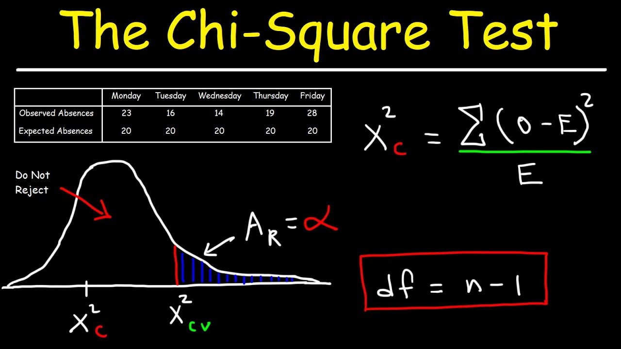
The Chi-Square test statistic is calculated using the formula:
\(\chi^2 = \sum \frac{(O - E)^2}{E}\)
where:
- \(O\) = Observed frequency
- \(E\) = Expected frequency
Example
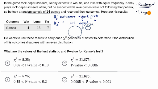
Suppose a shop owner claims that an equal number of customers come into the shop each weekday. An independent researcher records the number of customers over one week as follows:
| Monday | 50 |
| Tuesday | 60 |
| Wednesday | 40 |
| Thursday | 47 |
| Friday | 53 |
To perform the Chi-Square Goodness of Fit test:
- Calculate the expected frequency for each day: \(E = \frac{250}{5} = 50\).
- Calculate \((O - E)^2 / E\) for each day:
- Monday: \((50-50)^2/50 = 0\)
- Tuesday: \((60-50)^2/50 = 2\)
- Wednesday: \((40-50)^2/50 = 2\)
- Thursday: \((47-50)^2/50 = 0.18\)
- Friday: \((53-50)^2/50 = 0.18\)
- Sum these values to get the test statistic: \(\chi^2 = 0 + 2 + 2 + 0.18 + 0.18 = 4.36\).
Using the Chi-Square distribution table, compare the test statistic with the critical value to determine if the null hypothesis can be rejected.
Conclusion
If the p-value is less than the chosen significance level (e.g., 0.05), reject the null hypothesis. Otherwise, fail to reject the null hypothesis, indicating that the sample data does not provide sufficient evidence to conclude that the observed distribution differs from the expected distribution.
Applications
- Testing if a die is fair.
- Determining if the distribution of M&M colors is uniform.
- Evaluating if customer visits to a store are consistent across weekdays.
READ MORE:
Introduction to Chi-Square Goodness of Fit Test
The Chi-Square Goodness of Fit Test is a statistical method used to determine if a sample data set matches an expected distribution. This test is widely used in various fields such as genetics, marketing, and social sciences to analyze categorical data. The test compares the observed frequencies in each category to the frequencies that would be expected if the null hypothesis were true. The formula for the chi-square statistic is:
\[
\chi^2 = \sum \frac{(O_i - E_i)^2}{E_i}
\]
where \(O_i\) represents the observed frequency for category \(i\) and \(E_i\) represents the expected frequency for category \(i\).
Below is a step-by-step guide to performing the Chi-Square Goodness of Fit Test:
- State the hypotheses:
- Null hypothesis (\(H_0\)): The observed frequencies fit the expected distribution.
- Alternative hypothesis (\(H_a\)): The observed frequencies do not fit the expected distribution.
- Calculate the expected frequencies for each category based on the total sample size and the expected proportions.
- Compute the chi-square statistic using the formula above.
- Determine the degrees of freedom, which is the number of categories minus one.
- Find the critical value from the chi-square distribution table using the degrees of freedom and the chosen significance level (typically 0.05).
- Compare the computed chi-square statistic to the critical value to determine whether to reject the null hypothesis.
Example: Suppose a company wants to test if the distribution of colors in a package of M&Ms matches the expected distribution. They collect a sample and record the following observed frequencies: 212 blue, 147 orange, 103 green, 50 red, 46 yellow, and 42 brown. The expected frequency for each color is \( \frac{1}{6} \times 600 = 100 \). Using the formula, they calculate the chi-square statistic and compare it to the critical value to determine if the observed distribution significantly differs from the expected distribution.
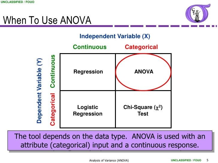
When to Use the Chi-Square Goodness of Fit Test
The Chi-Square Goodness of Fit Test is a statistical method used to determine if a sample data set matches a population with a specific distribution. Here are the key scenarios and conditions for using this test:
- The variable under study is categorical.
- The data is obtained through simple random sampling.
- The expected frequency count for each category is at least 5.
This test is ideal for situations where you want to compare the observed frequencies in different categories with the frequencies that are expected under a specific hypothesis. For example:
- Testing if a die is fair by comparing the observed frequency of each face to the expected frequency.
- Determining if a set of sample data follows a known distribution, such as a normal distribution.
- Validating assumptions in genetics about the distribution of different phenotypes.
The process involves four main steps:
- State the null and alternative hypotheses. The null hypothesis (H0) typically states that the sample data fits the expected distribution, while the alternative hypothesis (H1) states that it does not.
- Determine the expected frequencies for each category.
- Calculate the chi-square statistic using the formula: \[ \chi^2 = \sum \frac{(O_i - E_i)^2}{E_i} \] where \(O_i\) is the observed frequency and \(E_i\) is the expected frequency.
- Compare the chi-square statistic to a critical value from the chi-square distribution table to determine the p-value. If the p-value is less than the chosen significance level (e.g., 0.05), reject the null hypothesis.
This test is widely used in various fields such as biology, marketing, and social sciences to test hypotheses about distributions and ensure the validity of assumptions made based on categorical data.
Formulating Hypotheses
Formulating hypotheses is a crucial step in performing the Chi-Square Goodness of Fit Test. This test is used to determine if there is a significant difference between the observed frequencies and the expected frequencies in one or more categories. Here are the steps to formulate the null and alternative hypotheses:
-
Define the Null Hypothesis (\(H_0\)): The null hypothesis states that there is no significant difference between the observed and expected frequencies. It assumes that any difference is due to random chance. Formally, it can be written as:
\[ H_0: \text{The observed frequencies are equal to the expected frequencies.} \]
-
Define the Alternative Hypothesis (\(H_a\)): The alternative hypothesis states that there is a significant difference between the observed and expected frequencies. It suggests that the differences are not due to random chance. Formally, it can be written as:
\[ H_a: \text{The observed frequencies are not equal to the expected frequencies.} \]
For example, if we are testing whether a six-sided die is fair, our hypotheses would be:
- \( H_0: \) Each face of the die has an equal probability of \( \frac{1}{6} \).
- \( H_a: \) The probabilities of the faces are not all equal to \( \frac{1}{6} \).
These hypotheses set the stage for conducting the test by comparing the observed data to the expected distribution based on the null hypothesis.
Calculating the Test Statistic
The Chi-Square Goodness of Fit Test involves calculating a test statistic that measures the discrepancy between the observed and expected frequencies. Follow these steps to calculate the test statistic:
-
Step 1: Collect Data
Gather the observed frequencies (\( O_i \)) for each category from your sample data. Also, determine the expected frequencies (\( E_i \)) for each category based on the null hypothesis.
-
Step 2: Calculate the Chi-Square Statistic
Use the formula for the Chi-Square statistic:
\[ \chi^2 = \sum_{i=1}^{n} \frac{(O_i - E_i)^2}{E_i} \]
Where:
- \( O_i \) = Observed frequency for category \( i \)
- \( E_i \) = Expected frequency for category \( i \)
- \( n \) = Number of categories
Perform the following calculations for each category:
- Subtract the expected frequency from the observed frequency: \( O_i - E_i \)
- Square the result: \( (O_i - E_i)^2 \)
- Divide the squared difference by the expected frequency: \( \frac{(O_i - E_i)^2}{E_i} \)
Sum these values for all categories to obtain the Chi-Square statistic (\( \chi^2 \)).
-
Step 3: Example Calculation
Consider an example where we roll a six-sided die 60 times. The observed frequencies are as follows:
Face Observed Frequency (\( O_i \)) Expected Frequency (\( E_i \)) \( (O_i - E_i)^2 \) \( \frac{(O_i - E_i)^2}{E_i} \) 1 8 10 4 0.4 2 12 10 4 0.4 3 9 10 1 0.1 4 11 10 1 0.1 5 10 10 0 0 6 10 10 0 0 Summing the values in the last column gives us the Chi-Square statistic:
\[ \chi^2 = 0.4 + 0.4 + 0.1 + 0.1 + 0 + 0 = 1.0 \]
Thus, the Chi-Square statistic for this example is 1.0. This value will be used to determine the significance of the results by comparing it to a critical value from the Chi-Square distribution table.

Degrees of Freedom
The degrees of freedom (df) in a Chi-Square Goodness of Fit Test are a crucial component in determining the critical value against which the test statistic will be compared. The degrees of freedom are calculated based on the number of categories being analyzed. Here's how you can determine the degrees of freedom for your test:
-
Step 1: Count the Number of Categories
Identify the total number of categories (\( k \)) in your data set. Each category represents a possible outcome.
-
Step 2: Apply the Degrees of Freedom Formula
The formula for calculating the degrees of freedom in a Chi-Square Goodness of Fit Test is:
\[ df = k - 1 \]
Where:
- \( k \) = Total number of categories
-
Step 3: Example Calculation
Consider the example of a six-sided die. There are 6 possible outcomes (categories), so the degrees of freedom would be calculated as follows:
\[ df = 6 - 1 = 5 \]
To summarize, the degrees of freedom for the Chi-Square Goodness of Fit Test are equal to the number of categories minus one. This value is used to find the critical value from the Chi-Square distribution table, which is necessary to interpret the test statistic and determine the significance of the results.
Using the Chi-Square Distribution Table
After calculating the Chi-Square test statistic and determining the degrees of freedom, the next step is to use the Chi-Square distribution table to find the critical value. This critical value helps in deciding whether to reject the null hypothesis. Follow these steps to use the Chi-Square distribution table:
-
Step 1: Determine the Significance Level
Choose a significance level (\( \alpha \)) for the test. Common significance levels are 0.05, 0.01, and 0.10. The significance level represents the probability of rejecting the null hypothesis when it is actually true (Type I error).
-
Step 2: Locate the Degrees of Freedom
Find the row in the Chi-Square distribution table that corresponds to the degrees of freedom (df) calculated in the previous section. The degrees of freedom are typically listed in the leftmost column of the table.
-
Step 3: Find the Critical Value
Within the row for the appropriate degrees of freedom, find the column that corresponds to your chosen significance level. The value at the intersection of this row and column is the critical value.
-
Step 4: Compare the Test Statistic to the Critical Value
Compare your calculated Chi-Square test statistic to the critical value from the table:
- If the test statistic is greater than the critical value, reject the null hypothesis (\( H_0 \)).
- If the test statistic is less than or equal to the critical value, do not reject the null hypothesis.
For example, if you have 5 degrees of freedom and a significance level of 0.05, the critical value from the Chi-Square distribution table is approximately 11.07. If your calculated test statistic is 12.5, you would reject the null hypothesis because 12.5 > 11.07.
Using the Chi-Square distribution table is essential for determining the statistical significance of your results, allowing you to draw meaningful conclusions from your Chi-Square Goodness of Fit Test.
Interpreting the Results
After calculating the Chi-Square test statistic and comparing it to the critical value from the Chi-Square distribution table, the next step is to interpret the results. This process involves determining whether the observed data significantly differ from the expected data. Here are the steps to interpret the results:
-
Step 1: Compare Test Statistic to Critical Value
Compare the Chi-Square test statistic (\( \chi^2 \)) to the critical value obtained from the Chi-Square distribution table.
- If \( \chi^2 \) is greater than the critical value, reject the null hypothesis (\( H_0 \)).
- If \( \chi^2 \) is less than or equal to the critical value, do not reject the null hypothesis.
-
Step 2: Make a Decision
- Rejecting the Null Hypothesis: If the test statistic is greater than the critical value, there is sufficient evidence to conclude that the observed frequencies significantly differ from the expected frequencies. This means that the differences are unlikely due to random chance, and the null hypothesis is rejected.
- Failing to Reject the Null Hypothesis: If the test statistic is less than or equal to the critical value, there is insufficient evidence to conclude that the observed frequencies significantly differ from the expected frequencies. This means that any differences are likely due to random chance, and the null hypothesis is not rejected.
-
Step 3: Interpret the Context
Interpret the statistical decision in the context of the research question or practical problem:
- Example: In the context of a six-sided die, if you reject the null hypothesis, you might conclude that the die is biased and does not produce each outcome with equal probability. If you fail to reject the null hypothesis, you might conclude that there is no evidence to suggest that the die is biased.
Interpreting the results of a Chi-Square Goodness of Fit Test allows you to draw meaningful conclusions about the data and understand whether observed deviations from expected frequencies are statistically significant.
Examples of Chi-Square Goodness of Fit Test
To illustrate the Chi-Square Goodness of Fit Test, let's consider a practical example.
Example: Distribution of M&M Colors
Suppose a researcher wants to determine if a standard package of M&Ms contains an equal number of each color. The colors are red, orange, yellow, green, blue, and brown. The null hypothesis is that each color is equally likely to occur.
- State the Hypotheses:
- \(H_0\): The proportions of all M&M colors are equal (\(p_1 = p_2 = \ldots = p_6 = \frac{1}{6}\)).
- \(H_1\): At least one color proportion is different.
- Collect Data:
Sample data from 600 M&Ms:
- Blue: 212
- Orange: 147
- Green: 103
- Red: 50
- Yellow: 46
- Brown: 42
- Calculate Expected Counts:
If the null hypothesis is true, each color should have \(\frac{600}{6} = 100\) M&Ms.
- Compute the Chi-Square Statistic:
Using the formula \(\chi^2 = \sum \frac{(O_i - E_i)^2}{E_i}\), where \(O_i\) are the observed counts and \(E_i\) are the expected counts:
- Blue: \(\frac{(212 - 100)^2}{100} = 125.44\)
- Orange: \(\frac{(147 - 100)^2}{100} = 22.09\)
- Green: \(\frac{(103 - 100)^2}{100} = 0.09\)
- Red: \(\frac{(50 - 100)^2}{100} = 25.00\)
- Yellow: \(\frac{(46 - 100)^2}{100} = 29.16\)
- Brown: \(\frac{(42 - 100)^2}{100} = 33.64\)
Sum of all: \(125.44 + 22.09 + 0.09 + 25.00 + 29.16 + 33.64 = 235.42\)
- Determine Degrees of Freedom:
Degrees of freedom (df) is \(k - 1\), where \(k\) is the number of categories. Here, \(df = 6 - 1 = 5\).
- Find the p-value:
Using a chi-square distribution table or calculator, the p-value for \(\chi^2 = 235.42\) with 5 degrees of freedom is extremely small (practically 0).
- Conclusion:
Since the p-value is less than the common significance level (e.g., 0.05), we reject the null hypothesis. There is strong evidence that the colors are not equally distributed in the M&M package.
Common Applications
The Chi-Square Goodness of Fit Test is widely used in various fields to determine whether observed data fits a specific distribution. Here are some common applications:
- Market Research:
Companies use this test to compare consumer preferences against expected preferences. For example, a retailer might want to know if the distribution of sales across different product categories matches the expected distribution based on market research.
- Genetics:
Geneticists use the test to verify if the distribution of genetic traits in a sample matches the expected distribution. For example, this test can be used to determine if the observed frequency of different genotypes fits the expected frequency predicted by Mendelian inheritance.
- Ecology:
Ecologists use the test to see if the distribution of species in different habitats fits an expected distribution. For instance, an ecologist might test whether the number of certain species in different areas of a forest matches what is expected based on the availability of resources.
- Manufacturing:
Manufacturers use the test to determine if the distribution of defects in products is consistent with a hypothesized distribution. This helps in quality control and ensuring that the production process is functioning as expected.
- Education:
In educational research, the test is used to compare the distribution of students' grades to an expected distribution. This can help educators understand if students' performance matches the expected outcomes based on their teaching methods.
These applications highlight the versatility of the Chi-Square Goodness of Fit Test in analyzing categorical data to assess how well observed distributions match theoretical expectations.
Limitations and Considerations
The Chi-Square Goodness of Fit Test is a powerful tool, but it comes with several limitations and considerations that must be taken into account to ensure accurate and meaningful results.
-
Sample Size:
The test requires a sufficiently large sample size to be valid. Small sample sizes can lead to inaccurate results. As a general rule, all expected frequencies should be at least 5.
-
Expected Frequency:
At least 80% of the expected frequencies should be greater than 5. If this assumption is violated, the chi-square test may not be appropriate, and you may need to combine categories to increase the expected frequencies.
-
Independence of Observations:
The observations must be independent of each other. The test is not valid if there is any form of dependence between observations.
-
Applicability to Categorical Data:
The test is designed for categorical data. It is not suitable for continuous data, unless the data can be categorized meaningfully.
-
Sensitivity to Sample Size:
The chi-square statistic is sensitive to the sample size. With very large samples, even small differences between observed and expected frequencies can become statistically significant, which may not be practically significant.
-
Zero Frequencies:
If any expected frequency is zero, the chi-square test cannot be used. This issue can sometimes be mitigated by combining categories.
-
Assumption of Distribution:
The chi-square test assumes that the data follows a specific distribution. If this assumption is incorrect, the results of the test may not be valid.
-
Combining Categories:
If some categories have very low frequencies, it may be necessary to combine them to meet the test's assumptions. However, this should be done carefully to avoid losing important information.
In conclusion, while the Chi-Square Goodness of Fit Test is a useful statistical tool, it is important to be aware of its limitations and to ensure that its assumptions are met. Careful consideration of these factors will help to ensure that the results of the test are valid and meaningful.
Kiểm Định Chi-Square
READ MORE:
Video hướng dẫn về kiểm định sự phù hợp chi-square, giúp bạn hiểu rõ hơn về cách thực hiện và áp dụng phương pháp này.
Kiểm Định Sự Phù Hợp Chi-Square
:max_bytes(150000):strip_icc()/Chi-SquareStatistic_Final_4199464-7eebcd71a4bf4d9ca1a88d278845e674.jpg)