Topic expected value of x squared: The concept of the expected value of \(X^2\) is pivotal in statistics and probability theory. It extends the basic idea of expected value to non-linear functions, providing insights into the variability and distribution of a random variable's squared values. This article will guide you through its definition, calculation methods, and applications.
Table of Content
- Expected Value of \(X^2\)
- Introduction
- Definition of Expected Value
- Mathematical Formulation
- Expected Value of X Squared
- Applications in Probability and Statistics
- Examples and Solved Problems
- Expected Value in Various Distributions
- Relation to Variance and Standard Deviation
- Historical Background and Development
- Advanced Topics and Further Reading
- YOUTUBE: Video về giá trị kỳ vọng và phương sai của các biến ngẫu nhiên rời rạc, giải thích khái niệm và các ví dụ minh họa.
Expected Value of \(X^2\)
The expected value of a random variable \(X^2\), denoted as \(E(X^2)\), is a fundamental concept in probability and statistics. It is calculated differently depending on whether the random variable is discrete or continuous.
Discrete Random Variable
For a discrete random variable, the expected value of \(X^2\) can be calculated using the formula:
\[
E(X^2) = \sum_{i} x_i^2 \cdot P(X = x_i)
\]
where \(x_i\) represents the possible values of the random variable \(X\), and \(P(X = x_i)\) is the probability that \(X\) takes the value \(x_i\).
Example Calculation
Consider a random variable \(X\) with the following probability distribution:
| \(X\) | 0 | 1 | 2 | 3 | 4 |
|---|---|---|---|---|---|
| \(P(X)\) | 0.1 | 0.2 | 0.3 | 0.25 | 0.15 |
The expected value of \(X^2\) is computed as follows:
\[
E(X^2) = (0^2 \cdot 0.1) + (1^2 \cdot 0.2) + (2^2 \cdot 0.3) + (3^2 \cdot 0.25) + (4^2 \cdot 0.15) = 0 + 0.2 + 1.2 + 2.25 + 2.4 = 6.05
\]
Continuous Random Variable
For a continuous random variable, the expected value of \(X^2\) is calculated using the integral:
\[
E(X^2) = \int_{-\infty}^{\infty} x^2 f(x) \, dx
\]
where \(f(x)\) is the probability density function of \(X\).
Properties of Expected Value
- The expected value of a constant is the constant itself.
- If \(X\) and \(Y\) are independent random variables, then \(E(XY) = E(X)E(Y)\).
- For any random variable \(X\), \(E(X^2) \geq (E(X))^2\). This is due to the fact that variance is non-negative.
Variance and Expected Value
Variance is a measure of the dispersion of a set of values. It is defined as:
\[
\text{Var}(X) = E(X^2) - (E(X))^2
\]
Thus, knowing \(E(X^2)\) and \(E(X)\) allows us to compute the variance of \(X\).
Examples and Applications
The concept of expected value of \(X^2\) is used extensively in various fields such as economics, finance, engineering, and natural sciences to assess risks, optimize processes, and model random phenomena.

READ MORE:
Introduction
The concept of the expected value, often denoted as \(E[X]\), is a fundamental idea in probability and statistics. It represents the average or mean value of a random variable over a large number of trials. When dealing with the expected value of \(X^2\), where \(X\) is a random variable, it provides insight into the distribution and variability of \(X\).
The expected value of \(X^2\), denoted as \(E[X^2]\), is particularly important in various applications, including finance, engineering, and the natural sciences. It helps in understanding the dispersion or spread of values around the mean, which is crucial for risk assessment and decision-making processes.
Mathematically, \(E[X^2]\) can be computed using the probability distribution of \(X\). For a discrete random variable, it is calculated as:
\[
E[X^2] = \sum_{i} p(x_i) x_i^2
\]
where \(p(x_i)\) is the probability of \(X\) taking the value \(x_i\). For a continuous random variable, it is computed as:
\[
E[X^2] = \int_{-\infty}^{\infty} x^2 f(x) dx
\]
where \(f(x)\) is the probability density function of \(X\).
Understanding \(E[X^2]\) is also essential for calculating the variance of \(X\), which is given by:
\[
\text{Var}(X) = E[X^2] - (E[X])^2
\]
This relationship shows that the variance is the expected value of the squared deviation from the mean, providing a measure of how spread out the values of \(X\) are around the mean.
Definition of Expected Value
The expected value, often denoted as \( \mathbb{E}[X] \) for a random variable \( X \), is a fundamental concept in probability and statistics. It represents the long-term average or mean value of a random variable over numerous trials or experiments.
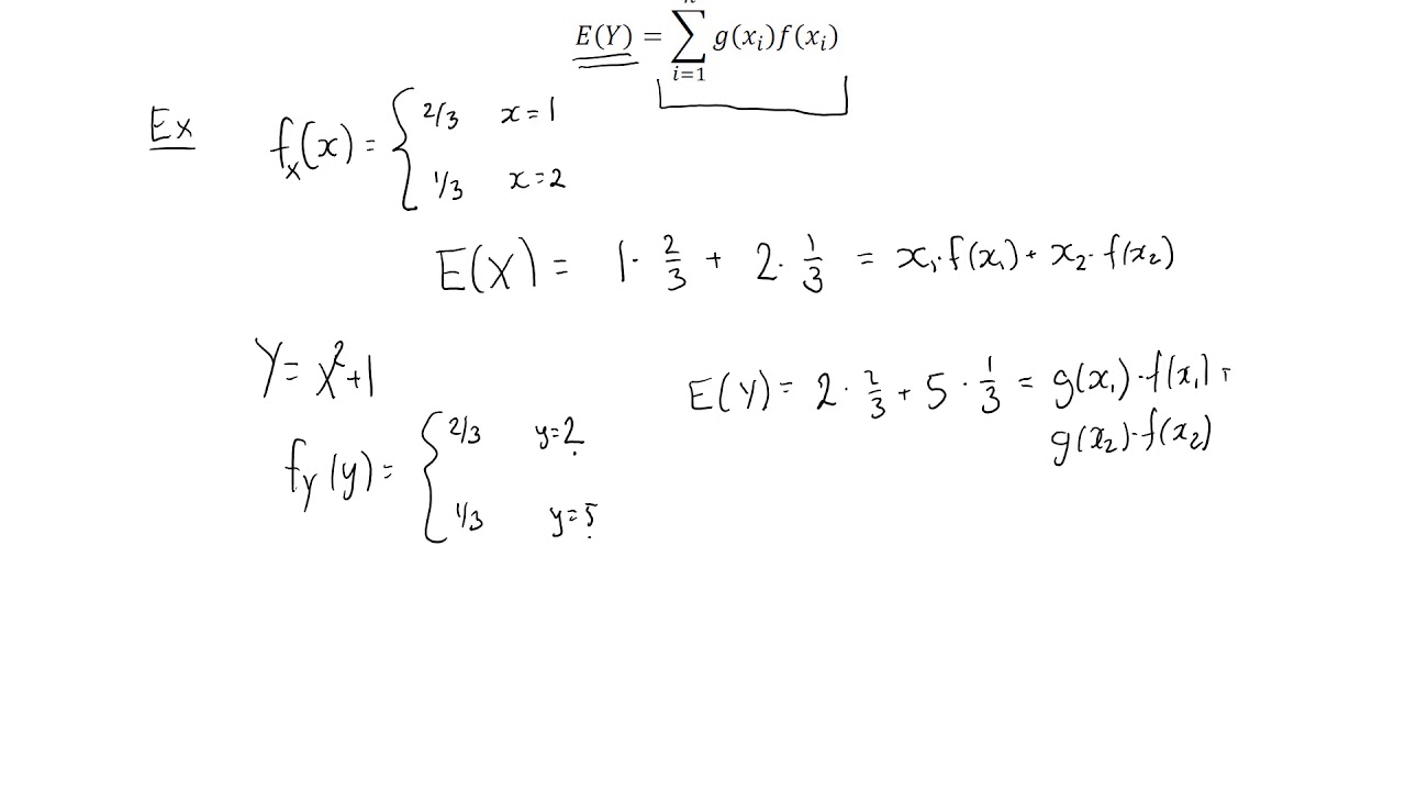
Mathematically, if \( X \) is a discrete random variable with possible values \( x_1, x_2, \ldots, x_n \) and corresponding probabilities \( p_1, p_2, \ldots, p_n \), the expected value is calculated as:
\[ \mathbb{E}[X] = \sum_{i=1}^{n} x_i p_i \]
For a continuous random variable with a probability density function \( f(x) \), the expected value is given by the integral:
\[ \mathbb{E}[X] = \int_{-\infty}^{\infty} x f(x) \, dx \]
The expected value provides a measure of the center of the distribution of the variable, giving insight into its average outcome over many observations.
Mathematical Formulation
The expected value of \(X^2\), denoted as \(\mathbb{E}[X^2]\), can be formulated differently based on the nature of the random variable \(X\). Below, we outline the mathematical formulations for both discrete and continuous random variables.
Discrete Random Variables
For a discrete random variable \(X\) with a probability mass function (pmf) \(p(x)\), the expected value of \(X^2\) is calculated using the sum of the squared values multiplied by their respective probabilities:
\[ \mathbb{E}[X^2] = \sum_{x \in \text{Range}(X)} x^2 \cdot p(x) \]
For example, if \(X\) represents the outcome of a fair six-sided die, the expected value of \(X^2\) can be calculated as follows:
\[ \mathbb{E}[X^2] = \frac{1}{6}1^2 + \frac{1}{6}2^2 + \frac{1}{6}3^2 + \frac{1}{6}4^2 + \frac{1}{6}5^2 + \frac{1}{6}6^2 = 15.17 \]
Continuous Random Variables
For a continuous random variable \(X\) with a probability density function (pdf) \(f(x)\), the expected value of \(X^2\) is calculated using the integral of the squared values multiplied by their respective probabilities:
\[ \mathbb{E}[X^2] = \int_{-\infty}^{\infty} x^2 f(x) \, dx \]
Consider a continuous random variable with the pdf:
\[ f(x) = \begin{cases}
\frac{3}{8}(6x - x^2) & 0 \leq x \leq 1 \\
0 & \text{otherwise}
\end{cases}
\]
We then calculate the expected value of \(X^2\) over the interval \([0, 1]\):
\[ \mathbb{E}[X^2] = \int_0^1 x^2 \cdot \frac{3}{8}(6x - x^2) \, dx = \int_0^1 \left(\frac{18}{8}x^3 - \frac{3}{8}x^4\right) dx \]
Evaluating this integral yields:
\[ \mathbb{E}[X^2] = \left[ \frac{18}{32} x^4 - \frac{3}{40} x^5 \right]_0^1 = \frac{18}{32} - \frac{3}{40} = 0.56 \]
Summary
- For discrete variables, sum the squared values multiplied by their probabilities.
- For continuous variables, integrate the squared values multiplied by their pdf over the defined range.
Expected Value of X Squared
The expected value of \(X^2\) is a crucial concept in probability and statistics, providing insights into the variance and overall distribution of a random variable. Formally, the expected value of \(X^2\) for a random variable \(X\) is defined as \(E(X^2)\). This can be calculated using the probability distribution of \(X\) and involves summing or integrating the squared values of \(X\) weighted by their probabilities.
For a discrete random variable \(X\) with possible values \(x_i\) and probabilities \(P(x_i)\), the expected value of \(X^2\) is given by:
\[ E(X^2) = \sum_{i} x_i^2 \cdot P(x_i) \]
In the case of a continuous random variable, the expected value of \(X^2\) is computed using the integral:
\[ E(X^2) = \int_{-\infty}^{\infty} x^2 \cdot f(x) \, dx \]
where \(f(x)\) is the probability density function of \(X\).
Understanding \(E(X^2)\) is essential for deriving other statistical measures, such as the variance of \(X\). The variance, \(Var(X)\), is related to the expected value of \(X\) and \(X^2\) through the formula:
\[ Var(X) = E(X^2) - [E(X)]^2 \]
This relationship highlights the importance of \(E(X^2)\) in capturing the spread and variability of the random variable \(X\).
Applications in Probability and Statistics
The expected value of \(X^2\) is a critical concept in probability and statistics with numerous applications. Understanding the expected value helps in predicting average outcomes and making informed decisions based on probabilistic models.
- Variance Calculation: The expected value of \(X^2\) is integral in computing the variance of a random variable \(X\). Variance is given by \( \text{Var}(X) = \mathbb{E}[X^2] - (\mathbb{E}[X])^2 \), providing a measure of how spread out the values of \(X\) are around the mean.
- Central Limit Theorem: The expected value of squared random variables plays a role in the Central Limit Theorem, which states that the sum of a large number of independent and identically distributed random variables tends to be normally distributed, regardless of the original distribution.
- Risk Management: In finance, the expected value of \(X^2\) is used to assess risk and volatility of assets. For instance, in portfolio management, it's used to calculate the variance and standard deviation of returns, which are crucial for risk assessment.
- Moment Generating Functions: The second moment (expected value of \(X^2\)) is used in moment generating functions to characterize the distribution of random variables, providing insights into their properties and behavior.
- Hypothesis Testing: In statistical hypothesis testing, the expected value of \(X^2\) is used in test statistics, such as chi-square tests, to determine the goodness of fit and independence in categorical data.
Examples and Solved Problems
Here are some examples and solved problems to illustrate the concept of the expected value of \(X^2\).
Example 1: Discrete Random Variable
Consider a discrete random variable \(X\) with the following probability distribution:
| X | 0 | 1 | 2 | 3 | 4 | 5 | 6 |
|---|---|---|---|---|---|---|---|
| p(X) | 0.06 | 0.15 | 0.17 | 0.24 | 0.23 | 0.09 | 0.06 |
To calculate \(E(X^2)\), use the formula:
\[
E(X^2) = \sum (x^2 \cdot p(x))
\]
Calculating step-by-step:
\[
E(X^2) = (0)^2 \cdot 0.06 + (1)^2 \cdot 0.15 + (2)^2 \cdot 0.17 + (3)^2 \cdot 0.24 + (4)^2 \cdot 0.23 + (5)^2 \cdot 0.09 + (6)^2 \cdot 0.06
\]
\[
E(X^2) = 0 + 0.15 + 0.68 + 2.16 + 3.68 + 2.25 + 2.16 = 11.08
\]
Thus, the expected value of \(X^2\) is 11.08.
Example 2: Continuous Random Variable
For a continuous random variable \(X\) with probability density function \(f(x)\), the expected value of \(X^2\) is given by:
\[
E(X^2) = \int_{-\infty}^{\infty} x^2 f(x) \, dx
\]
Let's assume \(f(x)\) is a normal distribution with mean 0 and standard deviation 1. The integral simplifies to:
\[
E(X^2) = \int_{-\infty}^{\infty} x^2 \frac{1}{\sqrt{2\pi}} e^{-\frac{x^2}{2}} \, dx
\]
This integral evaluates to 1, so \(E(X^2) = 1\).
Example 3: Application in a Real-World Scenario
Consider a game where you roll a die, and the payout is the square of the outcome. What is the expected value of the payout?
The possible outcomes are 1, 2, 3, 4, 5, and 6, each with a probability of \(\frac{1}{6}\). Calculate \(E(X^2)\) as follows:
\[
E(X^2) = \frac{1}{6} (1^2 + 2^2 + 3^2 + 4^2 + 5^2 + 6^2)
\]
Performing the calculations:
\[
E(X^2) = \frac{1}{6} (1 + 4 + 9 + 16 + 25 + 36) = \frac{1}{6} \cdot 91 = 15.17
\]
So, the expected value of the payout is 15.17.
Example 4: Investment Decision
Suppose an investment gives you a 30% chance of making $60,000 and a 70% chance of losing $30,000. Calculate the expected value to decide whether to invest.
\[
E(X) = 0.3 \cdot 60000 + 0.7 \cdot (-30000)
\]
\[
E(X) = 18000 - 21000 = -3000
\]
Since the expected value is negative, it might be advisable not to invest.
Expected Value in Various Distributions
The concept of expected value applies across various probability distributions, each with its unique characteristics and formulas. Here we explore some common distributions and their expected values.
Uniform Distribution
For a uniform distribution over the interval \([a, b]\), the expected value is given by:
\[
E(X) = \frac{a + b}{2}
\]
This represents the midpoint of the interval.
Binomial Distribution
The expected value of a binomial distribution, where \(n\) is the number of trials and \(p\) is the probability of success in each trial, is calculated as:
\[
E(X) = n \cdot p
\]
This formula gives the average number of successes in \(n\) trials.
Geometric Distribution
For a geometric distribution with success probability \(p\), the expected value is:
\[
E(X) = \frac{1}{p}
\]
This indicates the average number of trials needed to get the first success.
Poisson Distribution
The expected value for a Poisson distribution with parameter \(\lambda\) (the rate of occurrences) is:
\[
E(X) = \lambda
\]
This represents the average number of occurrences in a given interval.
Exponential Distribution
For an exponential distribution with rate parameter \(\lambda\), the expected value is:
\[
E(X) = \frac{1}{\lambda}
\]
This gives the average time between occurrences.
Normal Distribution
The expected value (mean) of a normal distribution with mean \(\mu\) and standard deviation \(\sigma\) is simply:
\[
E(X) = \mu
\]
This is the central value around which the data is distributed.
Examples
- Uniform Distribution Example: If a random variable \(X\) is uniformly distributed between 2 and 8, then:
\[
E(X) = \frac{2 + 8}{2} = 5
\] - Binomial Distribution Example: For a binomial distribution with \(n = 10\) and \(p = 0.5\):
\[
E(X) = 10 \cdot 0.5 = 5
\] - Geometric Distribution Example: If the probability of success \(p = 0.25\):
\[
E(X) = \frac{1}{0.25} = 4
\] - Poisson Distribution Example: For a Poisson distribution with \(\lambda = 3\):
\[
E(X) = 3
\] - Exponential Distribution Example: If \(\lambda = 0.5\):
\[
E(X) = \frac{1}{0.5} = 2
\] - Normal Distribution Example: For a normal distribution with \(\mu = 50\):
\[
E(X) = 50
\]
These formulas and examples illustrate the computation of expected values in different distributions, highlighting the diverse applications of this fundamental concept in probability and statistics.
Relation to Variance and Standard Deviation
In probability and statistics, the expected value of \( X^2 \), denoted as \( E[X^2] \), plays a crucial role in understanding the variability of a random variable \( X \). Here’s how it relates to variance and standard deviation:
- Variance: The variance of a random variable \( X \), denoted as \( \text{Var}(X) \), is defined as \( \text{Var}(X) = E[(X - E[X])^2] \). Notice that this can be expanded using the square of \( X \): \[ \text{Var}(X) = E[X^2 - 2XE[X] + E[X]^2] = E[X^2] - (E[X])^2. \] Therefore, \[ E[X^2] = \text{Var}(X) + (E[X])^2. \] This formula illustrates that \( E[X^2] \) contributes to the variance of \( X \).
- Standard Deviation: The standard deviation \( \sigma_X \) of \( X \) is the square root of the variance: \[ \sigma_X = \sqrt{\text{Var}(X)} = \sqrt{E[X^2] - (E[X])^2}. \] Hence, \( E[X^2] \) directly influences the standard deviation of \( X \).
Understanding \( E[X^2] \) is essential for comprehending how spread out the values of \( X \) are around its mean \( E[X] \). It quantifies the average of the squares of the deviations from the mean, thereby providing insights into the variability of \( X \).

Historical Background and Development
The concept of expected value, including the expected value of \( X^2 \), has evolved significantly over time alongside the development of probability theory and statistics. Here are key points in its historical progression:
- Early Concepts: The notion of expected value traces back to the 17th century with contributions from mathematicians like Blaise Pascal and Pierre de Fermat, who laid foundational groundwork in probability theory.
- Rise of Probability Theory: In the 18th century, developments by figures such as Jacob Bernoulli, Abraham de Moivre, and Pierre-Simon Laplace expanded understanding of probability distributions and the concept of expected value.
- Formalization: The rigorous formulation of expected value as an integral part of probability theory came in the 19th century with the works of Carl Friedrich Gauss, Adolphe Quetelet, and others, who introduced mathematical rigor and formal definitions.
- Modern Era: Throughout the 20th century, expected value and its applications, including \( E[X^2] \), became fundamental in statistical analysis, decision theory, and various fields of applied mathematics.
- Contemporary Developments: Today, with the advent of computational statistics and advanced probabilistic modeling, the concept continues to evolve, playing a pivotal role in fields such as machine learning and data science.
The historical development of expected value underscores its enduring significance in shaping our understanding of uncertainty, variability, and decision-making processes in both theoretical and practical contexts.
Advanced Topics and Further Reading
Exploring the expected value of \( X^2 \) leads to deeper insights into advanced topics in probability and statistics. Here are some areas and resources for further study:
- Moment Generating Functions: Understanding how moments, including \( E[X^2] \), relate to moment generating functions provides a powerful tool for deriving distributions and properties of random variables.
- Central Limit Theorem: Exploring the implications of \( E[X^2] \) in relation to the central limit theorem elucidates how sums of independent random variables converge to normal distributions.
- Applications in Finance: Analyzing \( E[X^2] \) in financial models helps quantify risk and return, essential for portfolio optimization and derivative pricing.
- Bayesian Statistics: In Bayesian inference, \( E[X^2] \) plays a crucial role in updating beliefs and estimating parameters based on observed data.
- Machine Learning: Understanding \( E[X^2] \) informs the development of loss functions and evaluation metrics, critical for model training and performance assessment.
For further reading, delve into textbooks on probability theory, statistical inference, and specialized literature on topics such as stochastic processes and advanced mathematical statistics.
Video về giá trị kỳ vọng và phương sai của các biến ngẫu nhiên rời rạc, giải thích khái niệm và các ví dụ minh họa.
Giá trị kỳ vọng và phương sai của biến ngẫu nhiên rời rạc
READ MORE:
Biến Ngẫu Nhiên Rời Rạc - Giá Trị Kỳ Vọng của X và VarX


:max_bytes(150000):strip_icc()/Chi-SquareStatistic_Final_4199464-7eebcd71a4bf4d9ca1a88d278845e674.jpg)


