Topic chi squared variance: Discover the power of chi-squared variance in statistical analysis, a fundamental tool for comparing observed and expected frequencies. This essential concept helps determine goodness-of-fit, test independence, and analyze categorical data. Learn how chi-squared variance can transform your data interpretation and decision-making processes, providing deeper insights and more accurate results.
Table of Content
- Chi-Squared Variance
- Introduction to Chi-Squared Variance
- Understanding Chi-Squared Distribution
- Chi-Squared Test Formula and Calculation
- Applications of Chi-Squared Variance
- Goodness-of-Fit Test
- Test of Independence
- Variance Analysis in Categorical Data
- Steps to Perform a Chi-Squared Test
- Interpreting Chi-Squared Test Results
- Examples and Case Studies
- Common Pitfalls and Considerations
- Chi-Squared Test Assumptions
- Advanced Topics in Chi-Squared Variance
- Tools and Software for Chi-Squared Analysis
- Conclusion and Summary
- YOUTUBE: Video hướng dẫn chi tiết về kiểm tra phân phối chi-square đối với một phương sai hoặc độ lệch chuẩn, phù hợp cho việc học và nghiên cứu về phương sai chi bình phương.
Chi-Squared Variance
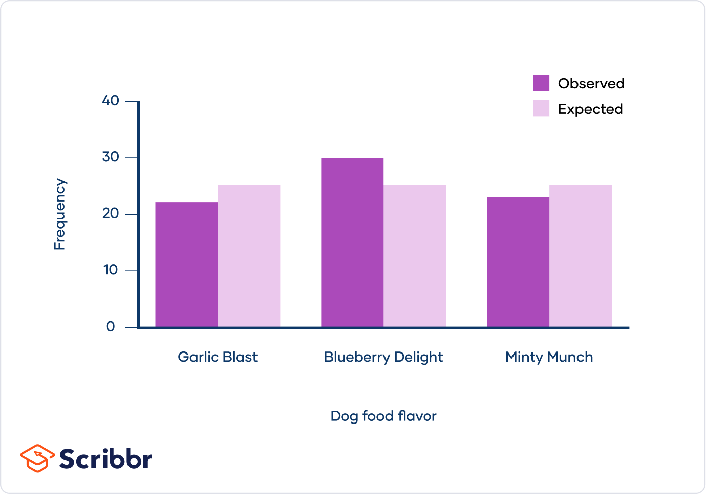
The chi-squared variance is a statistical concept that is used to measure the variability or dispersion of a set of observed data compared to expected data. It is commonly used in hypothesis testing and in the analysis of categorical data.
Overview
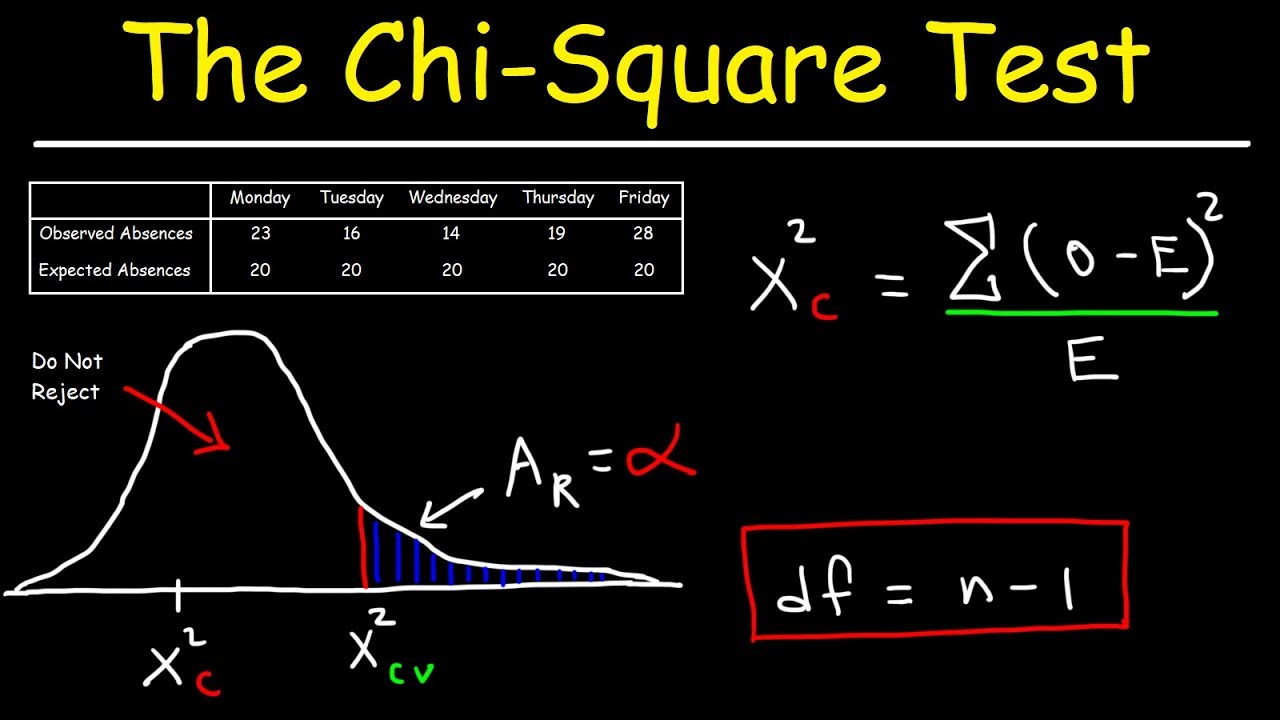
Chi-squared variance involves calculating the sum of the squared differences between observed and expected frequencies, divided by the expected frequencies. The formula for the chi-squared statistic is:
\[ \chi^2 = \sum \frac{(O_i - E_i)^2}{E_i} \]
where:
- \(\chi^2\) is the chi-squared statistic
- \(O_i\) is the observed frequency
- \(E_i\) is the expected frequency
Applications
Chi-squared variance is widely used in various fields including:
- Goodness-of-Fit Test: To determine how well a sample matches the expected distribution.
- Test of Independence: To assess whether two categorical variables are independent.
- Variance Analysis: To measure the dispersion in a set of categorical data.
Chi-Squared Distribution
The chi-squared distribution is a continuous probability distribution. It is used in hypothesis testing, particularly in tests of independence and goodness-of-fit. The distribution is characterized by its degrees of freedom (df), which are usually equal to the number of categories minus one.
The variance of the chi-squared distribution is:
\[ \text{Var}(\chi^2) = 2 \cdot \text{df} \]
Examples
Below is an example of how chi-squared variance can be used:
- Goodness-of-Fit Test:
Consider a dice roll experiment where you want to test if a die is fair. You roll the die 60 times and get the following observed frequencies for each face:
Face 1 2 3 4 5 6 Observed Frequency 8 12 10 11 9 10 The expected frequency for each face (assuming the die is fair) is 10. Using the chi-squared formula, you can calculate the chi-squared statistic to test the hypothesis.
- Test of Independence:
In a survey, you want to test if there is a relationship between gender and preference for a new product. The observed frequencies are recorded in a contingency table. You can use the chi-squared test to determine if the preference is independent of gender.

READ MORE:
Introduction to Chi-Squared Variance
Chi-squared variance is a fundamental concept in statistics used to assess how a set of observed data compares with expected data under a specified hypothesis. It is particularly useful in analyzing categorical data and determining the fit between observed frequencies and theoretical distributions. Here’s a detailed introduction:
The chi-squared test evaluates the discrepancies between observed and expected values across various categories, using the following formula:
\[ \chi^2 = \sum \frac{(O_i - E_i)^2}{E_i} \]
where:
- \( \chi^2 \) is the chi-squared statistic
- \( O_i \) represents the observed frequency
- \( E_i \) represents the expected frequency
This formula sums the squared differences between observed and expected values, each divided by the expected value, providing a measure of variance or deviation. The chi-squared test is used in two main scenarios:
- Goodness-of-Fit Test:
This test determines how well the observed frequencies of a single categorical variable match the expected frequencies. For example, it can assess whether a dice is fair by comparing the observed roll outcomes to the expected equal distribution across all faces.
- Test of Independence:
This test examines whether two categorical variables are independent. For instance, it can evaluate whether there is a relationship between gender and preference for a certain product by comparing the observed joint frequency distribution to the expected distribution under the assumption of independence.
The chi-squared distribution, used for these tests, depends on the degrees of freedom, calculated as:
\[ \text{df} = (r - 1)(c - 1) \]
where \( r \) is the number of rows and \( c \) is the number of columns in the contingency table. The shape of the chi-squared distribution varies based on these degrees of freedom, influencing the critical values used to assess the significance of the test results.
In summary, chi-squared variance provides a powerful method for analyzing the consistency of observed data with theoretical models or the independence of categorical variables. By understanding and applying this test, statisticians can make informed decisions based on empirical data.
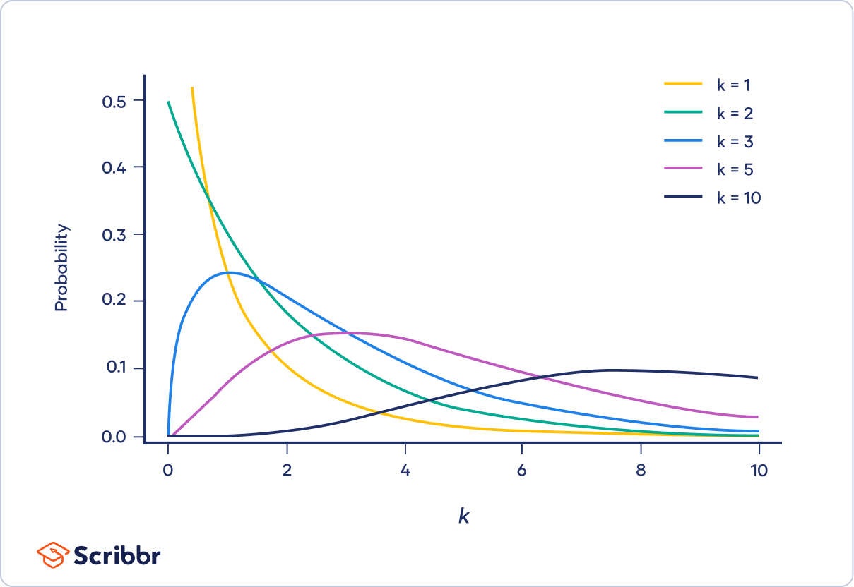
Understanding Chi-Squared Distribution
The chi-squared distribution is a critical concept in statistical analysis, commonly used for tests involving categorical data. It arises from the sum of the squares of independent standard normal random variables and plays a vital role in assessing the fit between observed and expected frequencies.
Here’s a detailed breakdown:
- Definition and Properties:
The chi-squared distribution with \( k \) degrees of freedom is defined as the distribution of a sum of the squares of \( k \) independent standard normal random variables. Mathematically:
\[ Y = \sum_{i=1}^{k} Z_i^2 \]where \( Z_i \) are independent standard normal variables \( (Z_i \sim N(0,1)) \). The resulting variable \( Y \) follows a chi-squared distribution \( \chi^2(k) \).
The key properties of the chi-squared distribution are:
- Mean: \( k \)
- Variance: \( 2k \)
- Skewness: \( \sqrt{8/k} \)
- Kurtosis: \( 12/k \)
- Degrees of Freedom:
The degrees of freedom (df) represent the number of independent pieces of information used to estimate a parameter. In a chi-squared test, the degrees of freedom are crucial for determining the distribution's shape and the critical values for hypothesis testing.
For a chi-squared goodness-of-fit test:
\[ \text{df} = k - 1 \]where \( k \) is the number of categories.
For a chi-squared test of independence:
\[ \text{df} = (r - 1)(c - 1) \]where \( r \) and \( c \) are the number of rows and columns in the contingency table.
- Chi-Squared Probability Density Function:
The probability density function (PDF) of the chi-squared distribution is given by:
\[ f(y; k) = \frac{1}{2^{k/2} \Gamma(k/2)} y^{(k/2)-1} e^{-y/2} \]for \( y > 0 \) and \( k \) degrees of freedom, where \( \Gamma \) is the gamma function.
- Applications:
The chi-squared distribution is primarily used in:
- Goodness-of-Fit Tests: To determine how well observed data fit an expected distribution.
- Tests of Independence: To assess if two categorical variables are independent in a contingency table.
- Variance Estimation: To estimate the variance of a population based on a sample variance.
- Examples:
Consider a study where we roll a six-sided die 60 times and observe the frequency of each outcome. To test if the die is fair, we use the chi-squared distribution to compare the observed frequencies with the expected frequencies (10 for each side if the die is fair).
In summary, understanding the chi-squared distribution allows for effective analysis of categorical data and the testing of hypotheses regarding distributions and independence. This distribution is fundamental in various statistical methods, providing robust tools for data analysis.
Chi-Squared Test Formula and Calculation
The chi-squared test is a statistical method used to compare observed frequencies in categorical data with expected frequencies based on a specific hypothesis. It is widely applied in tests of goodness-of-fit and independence. Below is a step-by-step guide to the chi-squared test formula and calculation:
- Formulate Hypotheses:
- Null Hypothesis (\( H_0 \)): Assumes that there is no significant difference between observed and expected frequencies.
- Alternative Hypothesis (\( H_1 \)): Assumes that there is a significant difference between observed and expected frequencies.
- Calculate Expected Frequencies:
The expected frequency for each category can be calculated using the formula:
\[ E_i = \frac{\text{Total observed} \times \text{Probability of category } i}{\text{Total number of categories}} \]In a contingency table, the expected frequency is given by:
\[ E_{ij} = \frac{( \text{Row total}_i \times \text{Column total}_j )}{\text{Grand total}} \] - Calculate Chi-Squared Statistic:
The chi-squared statistic is calculated using the formula:
\[ \chi^2 = \sum \frac{(O_i - E_i)^2}{E_i} \]where:
- \( O_i \) = observed frequency for category \( i \)
- \( E_i \) = expected frequency for category \( i \)
This formula calculates the sum of the squared differences between observed and expected frequencies, normalized by the expected frequencies.
- Determine Degrees of Freedom:
The degrees of freedom for the chi-squared test depend on the test type:
- Goodness-of-Fit Test:
\[ \text{df} = k - 1 \]where \( k \) is the number of categories.
- Test of Independence:
\[ \text{df} = (r - 1)(c - 1) \]where \( r \) is the number of rows and \( c \) is the number of columns in the contingency table.
- Goodness-of-Fit Test:
- Compare Chi-Squared Statistic to Critical Value:
Determine the critical value from the chi-squared distribution table based on the degrees of freedom and the chosen significance level (e.g., 0.05). Compare the calculated chi-squared statistic to the critical value:
- If \( \chi^2 \) < critical value, fail to reject the null hypothesis (\( H_0 \)).
- If \( \chi^2 \) ≥ critical value, reject the null hypothesis (\( H_0 \)).
Here’s an illustrative example:
| Category | Observed Frequency | Expected Frequency | (O - E)^2 | (O - E)^2 / E |
|---|---|---|---|---|
| A | 15 | 10 | 25 | 2.5 |
| B | 25 | 20 | 25 | 1.25 |
| C | 10 | 20 | 100 | 5.0 |
| D | 50 | 50 | 0 | 0 |
| Total | - | - | - | 8.75 |
In this example, the chi-squared statistic is 8.75. Based on the degrees of freedom and the chi-squared distribution table, you can determine whether to reject the null hypothesis.
In conclusion, the chi-squared test provides a methodical approach to analyzing categorical data, comparing observed frequencies against expected ones to draw meaningful conclusions.
Applications of Chi-Squared Variance
Chi-squared variance is a versatile statistical tool used in various fields to analyze categorical data and test hypotheses. Its primary applications include goodness-of-fit tests, tests of independence, and variance analysis. Here’s an in-depth look at its key applications:
- Goodness-of-Fit Test:
The chi-squared goodness-of-fit test assesses how well observed data fit a theoretical distribution. This test compares the observed frequencies with the expected frequencies across different categories to see if they deviate significantly from the expected model.
Steps:
- Formulate the null hypothesis (\( H_0 \)): The data follow the specified distribution.
- Calculate the expected frequencies based on the theoretical distribution.
- Compute the chi-squared statistic: \[ \chi^2 = \sum \frac{(O_i - E_i)^2}{E_i} \]
- Compare the chi-squared statistic to the critical value from the chi-squared distribution table.
Example: Testing if a die is fair by comparing observed roll outcomes to the expected equal distribution.
- Test of Independence:
The chi-squared test of independence determines if two categorical variables are independent or associated. It analyzes the relationship between variables by comparing the observed joint frequency distribution to the expected distribution assuming independence.
Steps:
- Formulate the null hypothesis (\( H_0 \)): The variables are independent.
- Create a contingency table of observed frequencies.
- Calculate the expected frequencies for each cell: \[ E_{ij} = \frac{(\text{Row total}_i \times \text{Column total}_j)}{\text{Grand total}} \]
- Compute the chi-squared statistic: \[ \chi^2 = \sum \frac{(O_{ij} - E_{ij})^2}{E_{ij}} \]
- Compare the chi-squared statistic to the critical value from the chi-squared distribution table.
Example: Evaluating whether there is a relationship between gender and product preference by analyzing survey data.
- Variance Analysis:
Chi-squared variance analysis is used to measure the variability in a set of categorical data. It helps in testing the homogeneity of variances across different groups or samples.
Steps:
- Calculate the sample variances for each group.
- Formulate the null hypothesis (\( H_0 \)): All groups have the same variance.
- Use the chi-squared test to compare the sample variances against the pooled variance.
Example: Testing if the variance in test scores across different classes is consistent.
- Other Applications:
Beyond the core tests, chi-squared variance is used in various domains:
- Model Fit Testing: Assessing the fit of models in machine learning and statistical analysis.
- Genetic Research: Analyzing the inheritance patterns in genetics to determine if they follow expected Mendelian ratios.
- Quality Control: Monitoring manufacturing processes to identify variations and maintain quality standards.
In summary, chi-squared variance is a robust and versatile tool in statistical analysis, allowing for thorough investigation and understanding of categorical data relationships and distributions. Its wide range of applications makes it invaluable in research, data analysis, and quality control.
Goodness-of-Fit Test
The goodness-of-fit test is a statistical procedure used to determine how well an observed frequency distribution matches an expected distribution. It assesses whether observed frequencies differ significantly from the frequencies expected under a specific theoretical distribution.
Here’s a detailed step-by-step guide to performing a goodness-of-fit test:
- Formulate Hypotheses:
- Null Hypothesis (\( H_0 \)): The observed frequencies fit the expected distribution.
- Alternative Hypothesis (\( H_1 \)): The observed frequencies do not fit the expected distribution.
- Collect and Organize Data:
Compile the observed frequencies for each category and calculate the expected frequencies based on the theoretical distribution. Ensure that the total of the expected frequencies matches the total of the observed frequencies.
- Calculate Expected Frequencies:
Determine the expected frequency for each category using the formula:
\[ E_i = N \times p_i \]where:
- \( N \) = total number of observations
- \( p_i \) = expected proportion for category \( i \)
- Compute the Chi-Squared Statistic:
Calculate the chi-squared statistic using the formula:
\[ \chi^2 = \sum \frac{(O_i - E_i)^2}{E_i} \]where:
- \( O_i \) = observed frequency for category \( i \)
- \( E_i \) = expected frequency for category \( i \)
- Determine Degrees of Freedom:
Calculate the degrees of freedom for the test using:
\[ \text{df} = k - 1 \]where \( k \) is the number of categories.
- Compare to Critical Value:
Compare the calculated chi-squared statistic to the critical value from the chi-squared distribution table based on the degrees of freedom and the chosen significance level (e.g., 0.05). Determine the critical value \( \chi^2_{\text{crit}} \).
- If \( \chi^2 < \chi^2_{\text{crit}} \), fail to reject the null hypothesis (\( H_0 \)).
- If \( \chi^2 \geq \chi^2_{\text{crit}} \), reject the null hypothesis (\( H_0 \)).
Example: Testing if a six-sided die is fair:
| Side | Observed Frequency | Expected Frequency | (O - E) | (O - E)^2 | (O - E)^2 / E |
|---|---|---|---|---|---|
| 1 | 8 | 10 | -2 | 4 | 0.4 |
| 2 | 12 | 10 | 2 | 4 | 0.4 |
| 3 | 9 | 10 | -1 | 1 | 0.1 |
| 4 | 11 | 10 | 1 | 1 | 0.1 |
| 5 | 10 | 10 | 0 | 0 | 0 |
| 6 | 10 | 10 | 0 | 0 | 0 |
| Total | 60 | 60 | - | 10 | 1.0 |
In this example, the chi-squared statistic is 1.0. Compare this value to the critical value from the chi-squared table with 5 degrees of freedom at the chosen significance level. Based on this comparison, decide whether to accept or reject the null hypothesis.
In conclusion, the goodness-of-fit test is a crucial method for evaluating how well observed data conform to a specified distribution. This test provides a framework for making statistical inferences about the fit between observed and expected data, essential for data analysis and decision-making.
Test of Independence
The chi-squared test of independence is a statistical method used to determine if there is a significant association between two categorical variables. It evaluates whether the distribution of sample data deviates from what would be expected under the assumption that the variables are independent.
Below is a comprehensive step-by-step guide to conducting a chi-squared test of independence:
- Formulate Hypotheses:
- Null Hypothesis (\( H_0 \)): The two variables are independent.
- Alternative Hypothesis (\( H_1 \)): The two variables are not independent.
- Collect and Organize Data:
Arrange the observed frequencies in a contingency table. Each cell in the table represents the frequency count for the combination of row and column variables.
- Calculate Expected Frequencies:
The expected frequency for each cell is calculated based on the marginal totals of the contingency table:
\[ E_{ij} = \frac{(\text{Row total}_i \times \text{Column total}_j)}{\text{Grand total}} \]where:
- \( E_{ij} \) = expected frequency for cell in row \( i \) and column \( j \)
- \( \text{Row total}_i \) = total of row \( i \)
- \( \text{Column total}_j \) = total of column \( j \)
- \( \text{Grand total} \) = sum of all frequencies in the table
- Compute the Chi-Squared Statistic:
Calculate the chi-squared statistic using the formula:
\[ \chi^2 = \sum \frac{(O_{ij} - E_{ij})^2}{E_{ij}} \]where:
- \( O_{ij} \) = observed frequency for cell in row \( i \) and column \( j \)
- \( E_{ij} \) = expected frequency for cell in row \( i \) and column \( j \)
- Determine Degrees of Freedom:
Calculate the degrees of freedom for the chi-squared statistic using:
\[ \text{df} = (r - 1)(c - 1) \]where \( r \) is the number of rows and \( c \) is the number of columns.
- Compare to Critical Value:
Compare the calculated chi-squared statistic to the critical value from the chi-squared distribution table based on the degrees of freedom and the chosen significance level (e.g., 0.05). Determine the critical value \( \chi^2_{\text{crit}} \).
- If \( \chi^2 < \chi^2_{\text{crit}} \), fail to reject the null hypothesis (\( H_0 \)).
- If \( \chi^2 \geq \chi^2_{\text{crit}} \), reject the null hypothesis (\( H_0 \)).
Example: Testing the independence between gender and voting preference:
| Gender | Preference A | Preference B | Total |
|---|---|---|---|
| Male | 30 | 20 | 50 |
| Female | 40 | 10 | 50 |
| Total | 70 | 30 | 100 |
Calculate the expected frequencies for each cell:
| Gender | Preference A | Preference B |
|---|---|---|
| Male | \( \frac{50 \times 70}{100} = 35 \) | \( \frac{50 \times 30}{100} = 15 \) |
| Female | \( \frac{50 \times 70}{100} = 35 \) | \( \frac{50 \times 30}{100} = 15 \) |
Compute the chi-squared statistic:
\[
\chi^2 = \sum \frac{(O_{ij} - E_{ij})^2}{E_{ij}} = \frac{(30 - 35)^2}{35} + \frac{(20 - 15)^2}{15} + \frac{(40 - 35)^2}{35} + \frac{(10 - 15)^2}{15} = 2.38
\]
Compare the calculated chi-squared value to the critical value with 1 degree of freedom. If 2.38 is less than the critical value, fail to reject the null hypothesis and conclude that gender and voting preference are independent. If it is greater, reject the null hypothesis and conclude that there is a significant association between gender and voting preference.
In conclusion, the chi-squared test of independence is an essential tool for analyzing the relationship between two categorical variables. It allows researchers to determine if the variables are independent or if there is a significant association between them, providing valuable insights in various fields such as sociology, marketing, and biology.
Variance Analysis in Categorical Data
Variance analysis in categorical data is a crucial aspect of statistical analysis, especially when dealing with categorical variables. The Chi-squared test is one of the primary methods used for this purpose. This test helps in understanding the distribution of categorical variables and determining if there are significant differences between expected and observed frequencies.
Here, we will discuss the steps involved in performing variance analysis in categorical data using the Chi-squared test:
-
Define Hypotheses
Start by defining the null hypothesis (H0) and the alternative hypothesis (Ha). The null hypothesis typically states that there is no significant difference between the observed and expected frequencies, while the alternative hypothesis suggests the opposite.
-
Collect Data
Gather the categorical data in a contingency table, which displays the frequency distribution of the variables. Ensure the data is comprehensive and accurately represents the population being studied.
-
Calculate Expected Frequencies
For each cell in the contingency table, calculate the expected frequency using the formula:
\[
E_{ij} = \frac{(R_i \times C_j)}{N}
\]
where \(E_{ij}\) is the expected frequency for cell \(i,j\), \(R_i\) is the total number of observations in row \(i\), \(C_j\) is the total number of observations in column \(j\), and \(N\) is the total number of observations. -
Compute the Chi-Squared Statistic
Use the formula to compute the Chi-squared statistic:
\[
\chi^2 = \sum \frac{(O_{ij} - E_{ij})^2}{E_{ij}}
\]
where \(O_{ij}\) is the observed frequency and \(E_{ij}\) is the expected frequency. -
Determine the Degrees of Freedom
Calculate the degrees of freedom (df) using the formula:
\[
df = (r-1) \times (c-1)
\]
where \(r\) is the number of rows and \(c\) is the number of columns. -
Compare with Critical Value
Compare the calculated Chi-squared statistic to the critical value from the Chi-squared distribution table, using the appropriate degrees of freedom and significance level (e.g., 0.05).
-
Interpret the Results
If the Chi-squared statistic exceeds the critical value, reject the null hypothesis. This indicates that there is a significant difference between the observed and expected frequencies.
The Chi-squared test for variance analysis in categorical data is a powerful tool for researchers. It allows for the examination of the relationships between categorical variables and aids in decision-making based on statistical evidence.
Steps to Perform a Chi-Squared Test
The Chi-squared test is a statistical method used to determine if there is a significant association between categorical variables. Here, we outline the detailed steps to perform a Chi-squared test:
-
State the Hypotheses
Formulate the null hypothesis (\(H_0\)) and the alternative hypothesis (\(H_a\)). The null hypothesis typically states that there is no association between the variables, while the alternative hypothesis indicates that an association exists.
-
Collect and Arrange Data
Collect data and organize it into a contingency table, showing the frequency distribution of the categorical variables.
Category 1 Category 2 Total Group 1 O11 O12 R1 Group 2 O21 O22 R2 Total C1 C2 N -
Calculate Expected Frequencies
Determine the expected frequencies for each cell using the formula:
\[
E_{ij} = \frac{R_i \times C_j}{N}
\]where \(E_{ij}\) is the expected frequency for cell \(i,j\), \(R_i\) is the total for row \(i\), \(C_j\) is the total for column \(j\), and \(N\) is the total sample size.
-
Compute the Chi-Squared Statistic
Calculate the Chi-squared statistic using the formula:
\[
\chi^2 = \sum \frac{(O_{ij} - E_{ij})^2}{E_{ij}}
\]where \(O_{ij}\) is the observed frequency and \(E_{ij}\) is the expected frequency for cell \(i,j\).
-
Determine Degrees of Freedom
Calculate the degrees of freedom (df) for the test using the formula:
\[
df = (r - 1) \times (c - 1)
\]where \(r\) is the number of rows and \(c\) is the number of columns in the contingency table.
-
Find the Critical Value
Refer to the Chi-squared distribution table to find the critical value at the desired significance level (e.g., 0.05) and degrees of freedom.
-
Compare and Make a Decision
Compare the calculated Chi-squared statistic with the critical value:
- If \(\chi^2\) is greater than the critical value, reject the null hypothesis, indicating a significant association between the variables.
- If \(\chi^2\) is less than or equal to the critical value, do not reject the null hypothesis, indicating no significant association between the variables.
-
Interpret the Results
Draw conclusions based on the decision made in the previous step. Summarize the findings and consider any practical implications or further research that may be needed.
Performing a Chi-squared test involves these systematic steps, ensuring a rigorous analysis of the relationship between categorical variables.

Interpreting Chi-Squared Test Results
Interpreting the results of a chi-squared test involves understanding the p-value, degrees of freedom, and the chi-squared statistic itself. Here is a detailed guide on how to interpret these results:
-
Calculate the Chi-Squared Statistic
The chi-squared statistic is calculated using the formula:
\[ \chi^2 = \sum \frac{(O - E)^2}{E} \]
Where \( O \) represents the observed frequencies and \( E \) represents the expected frequencies.
-
Determine the Degrees of Freedom
The degrees of freedom (df) for a chi-squared test are calculated based on the number of categories in your data:
\[ \text{df} = ( \text{number of rows} - 1 ) \times ( \text{number of columns} - 1 ) \]
-
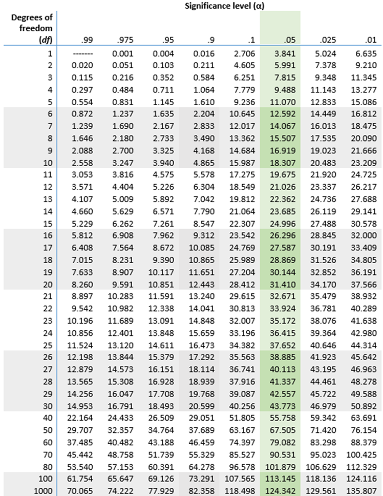
Find the Critical Value
Using a chi-squared distribution table, find the critical value for your calculated degrees of freedom and the chosen significance level (alpha, typically 0.05).
-
Compare the Chi-Squared Statistic to the Critical Value
If the chi-squared statistic is greater than the critical value from the table, you reject the null hypothesis. This indicates that there is a significant difference between the observed and expected frequencies.
-
Interpret the P-Value
The p-value indicates the probability that the observed results would occur by random chance. A smaller p-value (< 0.05) typically means the observed differences are statistically significant.
If \( p \leq 0.05 \), reject the null hypothesis.
If \( p > 0.05 \), do not reject the null hypothesis.
Let's break this down with an example:
Suppose you are testing whether a die is fair. You roll the die 60 times and record the number of times each face appears. Your observed frequencies might look like this:
| Face | Observed Frequency (O) | Expected Frequency (E) |
|---|---|---|
| 1 | 8 | 10 |
| 2 | 12 | 10 |
| 3 | 9 | 10 |
| 4 | 11 | 10 |
| 5 | 10 | 10 |
| 6 | 10 | 10 |
Using the chi-squared formula:
\[ \chi^2 = \frac{(8-10)^2}{10} + \frac{(12-10)^2}{10} + \frac{(9-10)^2}{10} + \frac{(11-10)^2}{10} + \frac{(10-10)^2}{10} + \frac{(10-10)^2}{10} \]
After calculating, you might find \( \chi^2 = 1.2 \).
With 5 degrees of freedom and an alpha of 0.05, the critical value from the chi-squared table is about 11.07.
Since 1.2 is less than 11.07, you do not reject the null hypothesis. The p-value is greater than 0.05, indicating no significant difference from what would be expected if the die were fair.
Examples and Case Studies
Chi-squared tests are widely used in various fields to determine if there is a significant association between categorical variables. Here are some detailed examples and case studies to illustrate the application of chi-squared tests.
Example 1: Testing a Die for Fairness
A researcher wants to determine if a six-sided die is fair. The die is rolled 60 times, and the outcomes are recorded as follows:
| Face | Observed Frequency |
|---|---|
| 1 | 10 |
| 2 | 8 |
| 3 | 12 |
| 4 | 11 |
| 5 | 9 |
| 6 | 10 |
The expected frequency for each face is 10 (since 60 rolls / 6 faces = 10). The chi-squared test statistic is calculated as:
\[
\chi^2 = \sum \frac{(O - E)^2}{E} = \frac{(10-10)^2}{10} + \frac{(8-10)^2}{10} + \frac{(12-10)^2}{10} + \frac{(11-10)^2}{10} + \frac{(9-10)^2}{10} + \frac{(10-10)^2}{10}
\]
\[
\chi^2 = 0 + 0.4 + 0.4 + 0.1 + 0.1 + 0 = 1
\]
With 5 degrees of freedom (number of categories - 1) and a significance level of 0.05, the critical value from the chi-squared table is 11.07. Since 1 < 11.07, we fail to reject the null hypothesis, indicating the die is fair.
Example 2: Customer Preference Survey
A store owner wants to know if customer preferences for three types of products (A, B, and C) are equally distributed. A survey of 150 customers yields the following results:
| Product | Observed Frequency |
|---|---|
| A | 60 |
| B | 50 |
| C | 40 |
The expected frequency for each product is 50 (since 150 customers / 3 products = 50). The chi-squared test statistic is calculated as:
\[
\chi^2 = \sum \frac{(O - E)^2}{E} = \frac{(60-50)^2}{50} + \frac{(50-50)^2}{50} + \frac{(40-50)^2}{50}
\]
\[
\chi^2 = \frac{100}{50} + 0 + \frac{100}{50} = 2 + 0 + 2 = 4
\]
With 2 degrees of freedom (number of categories - 1) and a significance level of 0.05, the critical value from the chi-squared table is 5.99. Since 4 < 5.99, we fail to reject the null hypothesis, indicating no significant difference in preferences among the three products.
Case Study: Education Level and Voting Behavior
Researchers want to determine if there is an association between education level (high school, college, postgraduate) and voting behavior (vote, did not vote) in a town. The data collected is as follows:
| Education Level | Voted | Did Not Vote |
|---|---|---|
| High School | 30 | 20 |
| College | 50 | 30 |
| Postgraduate | 40 | 10 |
The expected frequencies are calculated for each cell of the contingency table, and the chi-squared test statistic is calculated as:
\[
\chi^2 = \sum \frac{(O - E)^2}{E}
\]
After calculating the expected frequencies and the test statistic, the critical value is determined based on the degrees of freedom (df = (rows - 1) * (columns - 1) = 2) and the significance level (0.05). The result is used to decide whether to reject the null hypothesis.
These examples and case studies illustrate how the chi-squared test can be applied in various real-world scenarios to test hypotheses about categorical data.
Common Pitfalls and Considerations
When performing a Chi-Squared test, it's essential to be aware of several common pitfalls and considerations to ensure the validity and accuracy of your results.
- Sample Size: A small sample size can lead to inaccurate results because the Chi-Squared test relies on the approximation of the sampling distribution to a Chi-Squared distribution. Ensure each expected frequency in your contingency table is at least 5 to maintain test validity.
- Expected Frequencies: The accuracy of the Chi-Squared test diminishes when expected frequencies are too low. If more than 20% of your expected frequencies are below 5, consider using Fisher's Exact Test as an alternative.
- Independence of Observations: The Chi-Squared test assumes that the observations are independent of each other. Dependencies within the data can lead to incorrect conclusions. Ensure that the data collection method supports the independence assumption.
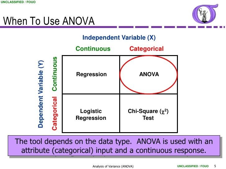
- Data Type: Chi-Squared tests are appropriate for categorical data. Using them with continuous data can lead to incorrect results. If you need to test continuous data, consider using other statistical tests such as t-tests or ANOVA.
- Null Hypothesis: Clearly define your null hypothesis before conducting the test. Misinterpretation of the null hypothesis can lead to incorrect inferences about your data.
- Multiple Testing: Be cautious when conducting multiple Chi-Squared tests on the same dataset. Each test increases the chance of a Type I error (false positive). Adjust your significance level using methods such as the Bonferroni correction to counteract this.
- Interpretation of Results: A significant result indicates that there is a difference between observed and expected frequencies, but it does not indicate the size or importance of the difference. Always consider the practical significance in addition to the statistical significance.
- Misleading Graphs and Tables: Ensure that any graphical or tabular representations of your data are clear and not misleading. Misrepresentation can lead to incorrect interpretations by the audience.
- Correct Degrees of Freedom: Accurately calculate the degrees of freedom for your test. For a goodness-of-fit test, degrees of freedom are calculated as \( df = k - 1 \), where \( k \) is the number of categories. For a test of independence, \( df = (r - 1) \times (c - 1) \), where \( r \) and \( c \) are the number of rows and columns in the contingency table.
By being mindful of these considerations, you can improve the reliability and validity of your Chi-Squared test results.
Chi-Squared Test Assumptions
When performing a Chi-Squared test, it is crucial to ensure that certain assumptions are met to validate the results. Here are the key assumptions for a Chi-Squared test:
- Independence of Observations: The observations must be independent of each other. This means the outcome of one observation does not influence another. Violations can occur in matched pair designs or repeated measures.
- Expected Frequency: Each expected frequency count in the contingency table should be 5 or more. If the expected frequency is less than 5 in more than 20% of the cells or any cell has an expected frequency of zero, the results may not be reliable. In such cases, using Fisher's exact test might be more appropriate.
- Sample Size: A sufficiently large sample size is required for the Chi-Squared approximation to be valid. Small sample sizes may lead to inaccurate conclusions due to a higher risk of Type II errors.
- Categorical Data: The Chi-Squared test is only applicable to categorical data. Continuous data must be categorized before applying the test.
- Random Sampling: The sample data should be randomly selected from the population to avoid biases and ensure the representativeness of the sample.
- No Zero Expected Frequencies: None of the cells in the contingency table should have an expected frequency of zero. If this condition is not met, the test results may be invalid.
- Mutually Exclusive Categories: The categories must be mutually exclusive, meaning each observation can only belong to one category.
By ensuring these assumptions are met, the Chi-Squared test can provide valid and reliable results for testing the independence of categorical variables.
Advanced Topics in Chi-Squared Variance
The chi-squared test is a powerful statistical tool used to assess the variance in categorical data. Beyond the basic applications, several advanced topics and extensions of the chi-squared test provide deeper insights and more nuanced analysis. Below are some advanced topics in chi-squared variance:
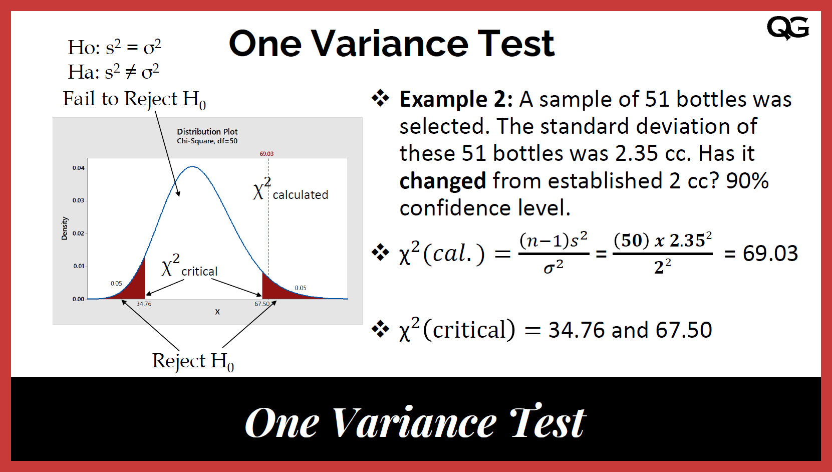
- Chi-Squared Test for Variance:
This test is used to determine whether the variance of a population is equal to a specified value. The test statistic is calculated as follows:
$$ \chi^2 = \frac{(n-1)s^2}{\sigma^2} $$
where \( n \) is the sample size, \( s^2 \) is the sample variance, and \( \sigma^2 \) is the population variance.
- Goodness-of-Fit Test:
This test evaluates whether a sample matches an expected distribution. It involves comparing observed frequencies with expected frequencies across categories. The test statistic is:
$$ \chi^2 = \sum \frac{(O_i - E_i)^2}{E_i} $$
where \( O_i \) is the observed frequency and \( E_i \) is the expected frequency for category \( i \).
- Test of Independence:
This test assesses whether two categorical variables are independent. It uses a contingency table to compare the expected frequencies under independence with the observed frequencies. The test statistic is:
$$ \chi^2 = \sum \frac{(O_{ij} - E_{ij})^2}{E_{ij}} $$
where \( O_{ij} \) is the observed frequency and \( E_{ij} \) is the expected frequency in the cell of row \( i \) and column \( j \).
- Adjustments for Small Sample Sizes:
When dealing with small sample sizes, the chi-squared test can be adjusted using Yates' correction for continuity. This reduces the chi-squared value slightly to account for the bias introduced by small samples:
$$ \chi^2 = \sum \frac{(|O_i - E_i| - 0.5)^2}{E_i} $$
- Monte Carlo Simulation:
For complex models or small sample sizes, Monte Carlo simulations can be used to approximate the distribution of the test statistic, providing more accurate p-values and confidence intervals.
- Likelihood-Ratio Test:
This test is an alternative to the chi-squared test and is particularly useful for nested models. It compares the likelihoods of the observed data under different hypotheses.
- Applications in Machine Learning:
Chi-squared tests are often used in feature selection for categorical data in machine learning. Features are selected based on their chi-squared statistics, helping to identify those most relevant to the target variable.
These advanced topics extend the utility of chi-squared tests, allowing for more comprehensive analysis and better decision-making based on categorical data.
Tools and Software for Chi-Squared Analysis
Several tools and software are available for performing Chi-Squared analysis, each offering unique features to facilitate statistical analysis. Below are some of the most commonly used tools:
- Python (SciPy and pandas): Python is a powerful programming language widely used in data analysis. The
SciPylibrary provides functions such asscipy.stats.chi2_contingencyfor performing Chi-Squared tests. Thepandaslibrary is useful for data manipulation and creating contingency tables. - R: R is a statistical software environment that offers comprehensive support for statistical analysis. Functions like
chisq.test()in base R and additional packages likevcdprovide tools for Chi-Squared tests and visualizations. - SPSS: SPSS (Statistical Package for the Social Sciences) is a user-friendly software for statistical analysis. It provides straightforward options for Chi-Squared tests through its menu-driven interface, making it accessible for users without programming knowledge.
- SAS: SAS is a software suite used for advanced analytics and statistical analysis. It includes procedures like
PROC FREQfor Chi-Squared tests, which are powerful for handling large datasets and complex analyses. - Excel: Microsoft Excel offers basic statistical functions, including Chi-Squared tests. With the Data Analysis Toolpak add-on, users can perform Chi-Squared tests through a simple, user-friendly interface.
- NCSS: NCSS provides comprehensive statistical and data analysis software. It offers tools specifically for Chi-Squared tests, contingency tables, and more advanced analysis, including detailed documentation and easy-to-read outputs.
- JASP: JASP is an open-source software designed for both classical and Bayesian statistical analysis. It offers an intuitive interface for Chi-Squared tests and other statistical analyses, making it accessible to beginners and experts alike.
Each of these tools offers different features and levels of complexity, making it possible for users of all skill levels to perform Chi-Squared analysis efficiently.
Conclusion and Summary
The chi-squared test is a powerful statistical tool used to assess the relationships between categorical variables. By comparing observed and expected frequencies, it helps determine whether any discrepancies are due to random chance or if they signify a meaningful pattern. Here is a concise summary of its key aspects and benefits:
- Purpose: Chi-squared tests are used for hypothesis testing, specifically to test the independence of variables and the goodness of fit of observed data to a theoretical model.
- Types of Chi-Squared Tests: The two primary types are the test of independence and the goodness-of-fit test.
- Assumptions: The test assumes that the data are from a random sample, variables are categorical, and expected frequencies in each cell are sufficiently large.
- Applications: Chi-squared tests are widely used in fields such as genetics, marketing, and social sciences to analyze categorical data.
- Limitations: Small sample sizes and low expected frequencies can invalidate the test results. Also, it is sensitive to the number of categories used.
In practice, chi-squared tests enable researchers to make informed decisions by statistically validating their hypotheses. For instance, they can determine if a new drug has a different effect on various demographic groups or if customer preferences for products are independent of their age groups.
Overall, the chi-squared test is an indispensable method in statistical analysis, providing a robust framework for understanding and interpreting categorical data.
Video hướng dẫn chi tiết về kiểm tra phân phối chi-square đối với một phương sai hoặc độ lệch chuẩn, phù hợp cho việc học và nghiên cứu về phương sai chi bình phương.
Kiểm Tra Phân Phối Chi-Square Đối Với Một Phương Sai Hoặc Độ Lệch Chuẩn
READ MORE:
Video về phương sai mẫu và phân phối chi bình phương. Khám phá cách tính toán và áp dụng phương sai mẫu trong các tình huống thực tế.
Phương Sai Mẫu và Phân Phối Chi Bình Phương
:max_bytes(150000):strip_icc()/Chi-SquareStatistic_Final_4199464-7eebcd71a4bf4d9ca1a88d278845e674.jpg)