Topic square root of neg 1: The square root of -1, known as the imaginary unit \(i\), is a fascinating concept that extends beyond real numbers. This article delves into its definition, properties, and applications, providing a comprehensive understanding of how imaginary numbers play a crucial role in advanced mathematics and various scientific fields.
Table of Content
- The Square Root of -1
- Introduction to Imaginary Numbers
- Definition and Properties of the Imaginary Unit
- Mathematical Representation of \(\sqrt{-1}\)
- The History and Development of Imaginary Numbers
- Applications of Imaginary Numbers in Various Fields
- Imaginary Numbers in Electrical Engineering
- Imaginary Numbers in Quantum Mechanics
- Visualizing Imaginary Numbers on the Complex Plane
- Complex Numbers and Their Components
- The Arithmetic of Complex Numbers
- Polar Form of Complex Numbers
- Euler's Formula and Its Significance
- Simplifying Expressions with Imaginary Numbers
- Solving Equations Using Imaginary Numbers
- Real-World Examples and Problem Solving
- Advanced Topics in Imaginary and Complex Numbers
- YOUTUBE:
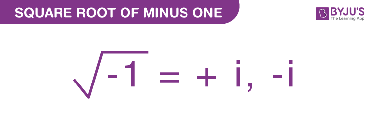
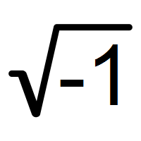
The Square Root of -1
The square root of -1 is a concept that extends beyond the real number system. In mathematics, the square root of -1 is defined as the imaginary unit, denoted as i.
Understanding Imaginary Numbers
Imaginary numbers are an extension of the real numbers and are used to solve equations that do not have real solutions. The imaginary unit i is defined by the property:
From this definition, it follows that:
\(\sqrt{-1} = i\)
Applications of Imaginary Numbers
- Complex Numbers: Imaginary numbers are used to form complex numbers, which are numbers of the form \(a + bi\), where \(a\) and \(b\) are real numbers.
- Electrical Engineering: Imaginary numbers are used to analyze AC circuits and signal processing.
- Quantum Mechanics: The mathematical framework of quantum mechanics heavily relies on complex numbers.
Properties of the Imaginary Unit
The imaginary unit i has some unique properties that differentiate it from real numbers:
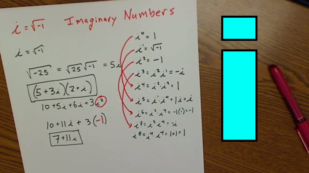
- Multiplication: \(i \times i = i^2 = -1\)
- Powers of i: The powers of i repeat in a cycle:
- \(i^1 = i\)
- \(i^2 = -1\)
- \(i^3 = -i\)
- \(i^4 = 1\)
- \(i^5 = i\)
- Complex Conjugate: The complex conjugate of \(a + bi\) is \(a - bi\).
Visualizing Imaginary Numbers
Imaginary numbers can be visualized using the complex plane, where the horizontal axis represents real numbers and the vertical axis represents imaginary numbers. A complex number \(a + bi\) is represented as a point \((a, b)\) in this plane.
For example, the number \(3 + 4i\) would be located 3 units along the real axis and 4 units along the imaginary axis.
Understanding and working with the square root of -1 and imaginary numbers opens up a wide range of mathematical and practical applications, making it a crucial concept in advanced mathematics and engineering.
READ MORE:
Introduction to Imaginary Numbers
Imaginary numbers are a fundamental concept in mathematics, extending the idea of real numbers to solve equations that have no real solutions. The key to understanding imaginary numbers lies in the imaginary unit, denoted as \(i\), which is defined by the property:
\(i^2 = -1\)
From this definition, the square root of -1 is expressed as:
\(\sqrt{-1} = i\)
Imaginary numbers were introduced to extend the solutions of polynomial equations. For example, the equation \(x^2 + 1 = 0\) has no real solution, but it has the solutions \(x = i\) and \(x = -i\) in the context of imaginary numbers.
Imaginary numbers are used in conjunction with real numbers to form complex numbers. A complex number is written in the form:
\(a + bi\)
where \(a\) and \(b\) are real numbers, and \(i\) is the imaginary unit. The number \(a\) is called the real part, and \(b\) is called the imaginary part of the complex number.
Here are some key points to understand imaginary numbers:
- Historical Context: Imaginary numbers were first conceptualized by mathematicians in the 16th century to solve cubic equations.
- Extension of Real Numbers: They extend the real number system to provide solutions to all polynomial equations.
- Complex Numbers: The combination of real and imaginary numbers forms complex numbers, which are essential in various fields of science and engineering.
Imaginary numbers are not just abstract concepts; they have practical applications in many areas, including electrical engineering, fluid dynamics, and quantum mechanics. They help in representing oscillations, waves, and other phenomena that vary with time.
To summarize, imaginary numbers expand our mathematical toolkit, allowing us to solve a broader range of problems and providing deeper insights into the nature of numbers and their applications.
Definition and Properties of the Imaginary Unit
The imaginary unit, denoted as \(i\), is a fundamental concept in mathematics that allows for the extension of the real number system to include solutions to equations that do not have real solutions. The imaginary unit is defined by the property:
\(i^2 = -1\)
This definition implies that the square root of -1 is represented as:
\(\sqrt{-1} = i\)
Here are the key properties and characteristics of the imaginary unit \(i\):
- Basic Powers of \(i\): The powers of \(i\) follow a cyclic pattern:
- \(i^1 = i\)
- \(i^2 = -1\)
- \(i^3 = -i\)
- \(i^4 = 1\)
- \(i^5 = i\), and the cycle repeats.
- Multiplication with Real Numbers: When multiplied by a real number, the imaginary unit \(i\) retains its properties. For example, \(3i\) represents a number that is three times the imaginary unit.
- Addition and Subtraction: Imaginary numbers can be added or subtracted in the same way as real numbers. For instance, \(2i + 3i = 5i\).
- Complex Conjugate: For a complex number \(a + bi\), the complex conjugate is \(a - bi\). This property is useful in simplifying expressions and solving equations.
Understanding these properties is crucial for working with complex numbers and performing various mathematical operations. Here is a table summarizing the powers of \(i\) and their results:
| Power of \(i\) | Result |
|---|---|
| \(i^1\) | \(i\) |
| \(i^2\) | \(-1\) |
| \(i^3\) | \(-i\) |
| \(i^4\) | 1 |
| \(i^5\) | \(i\) |
By understanding the definition and properties of the imaginary unit \(i\), we gain the ability to solve complex equations and explore advanced mathematical concepts, enriching our comprehension of the mathematical universe.
Mathematical Representation of \(\sqrt{-1}\)
The mathematical representation of the square root of -1, denoted as \(\sqrt{-1}\), is essential in extending the real number system to include imaginary and complex numbers. This representation is defined through the imaginary unit \(i\), which satisfies the equation:
\(i^2 = -1\)
Thus, the square root of -1 is represented as:
\(\sqrt{-1} = i\)
Here is a step-by-step explanation of how \(\sqrt{-1}\) is represented and used in mathematics:
- Definition: The imaginary unit \(i\) is defined by the property \(i^2 = -1\), leading to the fundamental representation \(\sqrt{-1} = i\).
- Complex Numbers: Imaginary numbers are combined with real numbers to form complex numbers, which are expressed in the form \(a + bi\), where \(a\) and \(b\) are real numbers. Here, \(a\) is the real part, and \(b\) is the imaginary part.
- Visual Representation: Complex numbers can be represented graphically on the complex plane, where the x-axis represents the real part, and the y-axis represents the imaginary part. For example, the complex number \(3 + 4i\) is represented as the point (3, 4).
- Operations with Complex Numbers: Various mathematical operations can be performed with complex numbers:
- Addition: \((a + bi) + (c + di) = (a + c) + (b + d)i\)
- Subtraction: \((a + bi) - (c + di) = (a - c) + (b - d)i\)
- Multiplication: \((a + bi)(c + di) = (ac - bd) + (ad + bc)i\)
- Division: \(\frac{a + bi}{c + di} = \frac{(a + bi)(c - di)}{c^2 + d^2} = \frac{ac + bd}{c^2 + d^2} + \frac{bc - ad}{c^2 + d^2}i\)
- Conjugate and Modulus: The complex conjugate of \(a + bi\) is \(a - bi\), and the modulus is \(\sqrt{a^2 + b^2}\). These are useful in simplifying expressions and solving equations involving complex numbers.
By understanding the mathematical representation of \(\sqrt{-1}\) as \(i\), we can explore the rich and diverse field of complex numbers, which has profound applications in engineering, physics, and various branches of mathematics.
The History and Development of Imaginary Numbers
The concept of imaginary numbers has a rich and fascinating history that spans several centuries. Imaginary numbers, particularly the square root of -1, were initially met with skepticism and confusion but eventually became a fundamental component of modern mathematics. Here is a detailed overview of their history and development:
- Early Beginnings:
- Imaginary numbers were first introduced in the 16th century by Italian mathematician Gerolamo Cardano. In his work "Ars Magna" (1545), Cardano encountered the square root of negative numbers while solving cubic equations, although he did not fully understand them.
- At this time, negative numbers themselves were not fully accepted, making the concept of imaginary numbers even more controversial.
- 17th Century Developments:
- In the 17th century, mathematicians like Rafael Bombelli made significant contributions to the understanding of imaginary numbers. Bombelli's work "L'Algebra" (1572) provided a more systematic approach to complex numbers, including rules for operations involving \(\sqrt{-1}\).
- Bombelli's efforts laid the groundwork for future acceptance and use of imaginary numbers.
- 18th Century Acceptance:
- During the 18th century, Leonhard Euler and Carl Friedrich Gauss played crucial roles in formalizing the use of imaginary numbers. Euler introduced the notation \(i\) for \(\sqrt{-1}\) and explored its properties extensively.
- Gauss furthered this work by developing the theory of complex numbers and proving the Fundamental Theorem of Algebra, which states that every polynomial equation has a solution in the complex numbers.
- 19th Century and Beyond:
- In the 19th century, William Rowan Hamilton introduced quaternions, extending the concept of complex numbers to higher dimensions. This period also saw the development of various applications of imaginary numbers in physics, engineering, and other sciences.
- Mathematicians continued to explore and expand the theory of complex numbers, leading to a deeper understanding and broader acceptance of imaginary numbers in mathematical analysis and applied fields.
Today, imaginary numbers are an integral part of mathematics, with applications in many scientific and engineering disciplines. Their development from a controversial concept to a fundamental mathematical tool highlights the dynamic and evolving nature of mathematical discovery.

Applications of Imaginary Numbers in Various Fields
Imaginary numbers, and more broadly complex numbers, have numerous applications across various fields of science and engineering. Here are some key areas where imaginary numbers play a crucial role:
- Electrical Engineering:
- Imaginary numbers are used extensively in the analysis of AC circuits. The impedance of an AC circuit, which combines resistance and reactance, is often expressed as a complex number \(Z = R + jX\), where \(j\) represents \(\sqrt{-1}\).
- Phasor analysis, which simplifies the study of oscillating signals, relies on complex numbers to represent sinusoidal functions as rotating vectors in the complex plane.
- Control Theory:
- In control systems engineering, the stability of systems is analyzed using complex numbers. The poles of the system's transfer function are located in the complex plane, and their positions determine system stability.
- Complex numbers are also used to design and analyze feedback loops and control responses.
- Quantum Mechanics:
- Imaginary numbers are fundamental in the mathematical framework of quantum mechanics. The Schrödinger equation, which describes the behavior of quantum particles, involves complex wave functions.
- Probability amplitudes, which determine the likelihood of a particle's state, are complex numbers whose magnitudes squared give real probabilities.
- Signal Processing:
- Complex numbers are used in Fourier transforms, which decompose signals into their constituent frequencies. The Fourier transform of a function \(f(t)\) is a complex function \(F(\omega)\) that provides frequency-domain information.
- Digital signal processing techniques often utilize complex numbers to filter, modulate, and demodulate signals.
- Fluid Dynamics:
- In fluid dynamics, complex potential functions are used to describe the flow of incompressible fluids. These functions simplify the analysis of flow patterns and velocity fields.
- The use of complex variables allows for the application of powerful mathematical techniques to solve problems involving fluid flow around objects.
- Vibration Analysis:
- Imaginary numbers are used in the study of mechanical vibrations and oscillations. The natural frequencies and modes of vibration of a system can be expressed using complex numbers.
- Analyzing the damping and resonant behavior of systems often involves complex arithmetic.
- Economics and Finance:
- In economics, complex numbers can model certain dynamic systems and cyclical behaviors in markets. Complex eigenvalues can indicate cyclical patterns in economic models.
- Financial models sometimes employ complex numbers in option pricing and other sophisticated financial instruments.
By extending the number system to include imaginary numbers, we gain powerful tools to solve a wide array of problems across different scientific and engineering disciplines. This versatility underscores the importance of imaginary numbers in both theoretical and applied mathematics.
Imaginary Numbers in Electrical Engineering
Imaginary numbers play a critical role in electrical engineering, particularly in the analysis and design of AC (alternating current) circuits. The use of imaginary numbers simplifies complex calculations and provides deeper insights into the behavior of electrical systems. Here is a detailed explanation of how imaginary numbers are used in electrical engineering:
- Impedance in AC Circuits:
- Impedance (\(Z\)) is a measure of opposition that a circuit presents to the passage of current when a voltage is applied. It combines resistance (\(R\)) and reactance (\(X\)) and is expressed as a complex number: \(Z = R + jX\), where \(j\) represents \(\sqrt{-1}\).
- Resistance (\(R\)) is the real part, representing energy dissipation, while reactance (\(X\)) is the imaginary part, representing energy storage in inductors and capacitors.
- Phasor Analysis:
- Phasors are a way to represent sinusoidal functions as rotating vectors in the complex plane. A sinusoidal voltage or current can be represented as a phasor: \(V = V_0 e^{j\omega t}\), where \(V_0\) is the amplitude, \(\omega\) is the angular frequency, and \(t\) is time.
- Phasor analysis simplifies the calculation of circuit parameters by transforming differential equations into algebraic equations in the complex domain.
- Power Calculations:
- Complex power (\(S\)) in AC circuits is represented as \(S = P + jQ\), where \(P\) is the real power (measured in watts) and \(Q\) is the reactive power (measured in volt-amperes reactive, VAR).
- Real power represents the actual energy consumed, while reactive power represents energy oscillating between the source and reactive components.
- Resonance and Frequency Response:
- Resonance in an electrical circuit occurs when the inductive reactance equals the capacitive reactance, resulting in a purely resistive impedance at a specific frequency. This condition can be analyzed using complex numbers.
- Frequency response analysis involves examining how the impedance or admittance of a circuit varies with frequency, often using complex functions to represent the behavior.
- Transfer Functions:
- Transfer functions, used to analyze the input-output relationship of a system, are expressed as complex functions of frequency. They provide a comprehensive understanding of the system's behavior in the frequency domain.
- For example, the transfer function \(H(j\omega)\) of a linear time-invariant (LTI) system can be used to determine the system's response to sinusoidal inputs.
In summary, imaginary numbers are indispensable in electrical engineering, providing a robust mathematical framework for analyzing and designing complex AC circuits. Their use simplifies calculations, enhances understanding, and enables engineers to solve a wide range of practical problems efficiently.
Imaginary Numbers in Quantum Mechanics
Imaginary numbers, particularly the imaginary unit \(i\) where \(i = \sqrt{-1}\), play a fundamental role in quantum mechanics. They are essential in the mathematical formulations that describe the behavior of quantum systems. One of the most critical uses of imaginary numbers in quantum mechanics is in the representation of wavefunctions.
The wavefunction, typically denoted as \(\psi\), is a complex-valued function that contains all the information about a quantum system. The square of the wavefunction's magnitude, \(|\psi|^2\), represents the probability density of finding a particle in a given state. Mathematically, the wavefunction can be written as:
\[
\psi(x, t) = A e^{i(kx - \omega t)}
\]
where \(A\) is the amplitude, \(k\) is the wave number, \(\omega\) is the angular frequency, and \(t\) is time. The presence of the imaginary unit \(i\) in the exponent is crucial for capturing the oscillatory nature of quantum states.
In quantum mechanics, the Schrödinger equation governs the evolution of the wavefunction. The time-dependent Schrödinger equation is given by:
\[
i\hbar \frac{\partial \psi}{\partial t} = \hat{H} \psi
\]
where \(\hbar\) is the reduced Planck constant, and \(\hat{H}\) is the Hamiltonian operator representing the total energy of the system. The imaginary unit \(i\) is essential for the equation to correctly describe the dynamics of the quantum system.
Imaginary numbers also play a vital role in quantum entanglement and superposition. In experiments involving entangled particles, the correlations between measurements can only be accurately described using complex numbers, which include imaginary components. For instance, in an entanglement-swapping experiment, complex-valued quantum theories provide predictions that align with observed results, whereas real-valued theories fail to do so.
Moreover, in quantum computing, qubits (quantum bits) are represented as complex vectors. Operations on qubits, such as quantum gates, often involve complex numbers to facilitate superpositions and entanglements that are essential for quantum algorithms.
In summary, imaginary numbers are indispensable in quantum mechanics. They enable accurate descriptions of quantum states, their evolution, and the intricate phenomena such as entanglement and superposition that define the quantum world.
Visualizing Imaginary Numbers on the Complex Plane
The complex plane is a powerful tool for visualizing complex numbers, where the horizontal axis represents the real part of the number and the vertical axis represents the imaginary part. This plane allows for a clear geometric interpretation of complex numbers.
Each complex number \( z \) can be expressed as \( z = a + bi \), where \( a \) is the real part and \( b \) is the imaginary part. On the complex plane, this number is represented by the point \((a, b)\).
Steps to Plot a Complex Number
- Identify the real part \( a \) and the imaginary part \( b \) of the complex number \( z = a + bi \).
- Move \( a \) units along the horizontal (real) axis.
- Move \( b \) units along the vertical (imaginary) axis.
- Plot the point \((a, b)\) on the complex plane.
For example, to plot the complex number \( 3 - 4i \):
- The real part is \( 3 \).
- The imaginary part is \( -4 \).
- Plot the point \((3, -4)\).
This point is three units to the right of the origin and four units down.
Magnitude and Argument
Two important concepts for visualizing complex numbers are the magnitude and the argument:
- Magnitude: The distance from the origin to the point \((a, b)\), calculated as \( |z| = \sqrt{a^2 + b^2} \).
- Argument: The angle \( \theta \) formed with the positive real axis, calculated using \( \theta = \tan^{-1}(\frac{b}{a}) \).
Example: Plotting Multiple Points
Consider plotting the complex numbers \( 1 + 2i \), \( -3 + 4i \), and \( -2 - 2i \) on the complex plane:
| Complex Number | Real Part | Imaginary Part | Point |
|---|---|---|---|
| \( 1 + 2i \) | 1 | 2 | \((1, 2)\) |
| \( -3 + 4i \) | -3 | 4 | \((-3, 4)\) |
| \( -2 - 2i \) | -2 | -2 | \((-2, -2)\) |
By plotting these points, we can easily visualize their positions relative to the real and imaginary axes. This helps in understanding the addition, subtraction, and multiplication of complex numbers geometrically.
Using the complex plane, we can also understand functions involving complex numbers, such as exponentiation, logarithms, and trigonometric functions, providing a deeper insight into their properties and behaviors.
For interactive visualization, tools like Desmos can be very helpful to dynamically plot and manipulate complex numbers on the plane.

Complex Numbers and Their Components
A complex number is a number of the form \(a + bi\), where \(a\) and \(b\) are real numbers, and \(i\) is the imaginary unit, defined by the property \(i^2 = -1\). The component \(a\) is called the real part of the complex number, and \(bi\) is called the imaginary part.
In mathematical notation:
- \(a\) is the real part: \(\text{Re}(a + bi) = a\)
- \(bi\) is the imaginary part: \(\text{Im}(a + bi) = b\)
Standard Form
Complex numbers are usually expressed in the standard form \(a + bi\). For example, \(5 + 3i\) is a complex number with real part 5 and imaginary part 3.
Operations with Complex Numbers
Just like real numbers, complex numbers can be added, subtracted, multiplied, and divided.
Addition and Subtraction
To add or subtract complex numbers, add or subtract their real parts and their imaginary parts separately:
- \((a + bi) + (c + di) = (a + c) + (b + d)i\)
- \((a + bi) - (c + di) = (a - c) + (b - d)i\)
Multiplication
To multiply complex numbers, use the distributive property and the fact that \(i^2 = -1\):
- \((a + bi)(c + di) = ac + adi + bci + bdi^2 = ac + adi + bci - bd = (ac - bd) + (ad + bc)i\)
Division
To divide complex numbers, multiply the numerator and the denominator by the conjugate of the denominator and simplify:
- \(\frac{a + bi}{c + di} \cdot \frac{c - di}{c - di} = \frac{(a + bi)(c - di)}{(c + di)(c - di)} = \frac{(ac + bd) + (bc - ad)i}{c^2 + d^2}\)
Complex Conjugates
The complex conjugate of a complex number \(a + bi\) is \(a - bi\). The product of a complex number and its conjugate is a real number:
- \((a + bi)(a - bi) = a^2 + b^2\)
Visualizing Complex Numbers
Complex numbers can be represented graphically on the complex plane, where the horizontal axis is the real axis and the vertical axis is the imaginary axis. A complex number \(a + bi\) is plotted as the point \((a, b)\) in this plane.
For example, the complex number \(3 - 4i\) is represented as the point \((3, -4)\).
The Arithmetic of Complex Numbers
Complex numbers, which take the form \( a + bi \) where \( a \) and \( b \) are real numbers and \( i \) is the imaginary unit (\( i^2 = -1 \)), can be manipulated using specific arithmetic rules. Below, we explore addition, subtraction, multiplication, and division of complex numbers.
Addition and Subtraction
Addition and subtraction of complex numbers are performed by combining the real and imaginary parts separately:
- Addition: \( (a + bi) + (c + di) = (a + c) + (b + d)i \)
- Subtraction: \( (a + bi) - (c + di) = (a - c) + (b - d)i \)
Multiplication
Multiplying complex numbers involves distributing the terms and applying the property \( i^2 = -1 \):
- For \( (a + bi)(c + di) \):
-
- Multiply the real parts: \( ac \)
- Multiply the outer and inner parts: \( adi + bci \)
- Multiply the imaginary parts: \( bdi^2 = -bd \)
- Combine the results: \( (ac - bd) + (ad + bc)i \)
- Example: \( (3 + 2i)(1 + 4i) = (3 \cdot 1 - 2 \cdot 4) + (3 \cdot 4 + 2 \cdot 1)i = -5 + 14i \)
Division
Dividing complex numbers involves multiplying the numerator and the denominator by the conjugate of the denominator to rationalize it:
- For \( \frac{a + bi}{c + di} \):
-
- Multiply by the conjugate: \( \frac{(a + bi)(c - di)}{(c + di)(c - di)} \)
- Simplify the denominator using \( (c + di)(c - di) = c^2 + d^2 \)
- Distribute and simplify the numerator
- Combine and separate the real and imaginary parts
- Example: \( \frac{3 + 2i}{1 - 4i} \):
- Conjugate: \( 1 + 4i \)
- Numerator: \( (3 + 2i)(1 + 4i) = 3 + 12i + 2i + 8i^2 = -5 + 14i \)
- Denominator: \( (1 - 4i)(1 + 4i) = 1 + 16 = 17 \)
- Result: \( \frac{-5 + 14i}{17} = -\frac{5}{17} + \frac{14}{17}i \)
Polar Form of Complex Numbers
The polar form of a complex number provides a different perspective from its rectangular form, which is represented as \( z = a + bi \). In the polar form, a complex number is expressed in terms of its magnitude (or modulus) and angle (or argument).
A complex number \( z \) can be represented as:
\( z = r (\cos \theta + i \sin \theta) \)
where:
- \( r \) is the magnitude of the complex number, given by \( r = \sqrt{a^2 + b^2} \)
- \( \theta \) is the argument of the complex number, given by \( \theta = \tan^{-1} \left( \frac{b}{a} \right) \)
The magnitude \( r \) is the distance of the point from the origin in the complex plane, and the argument \( \theta \) is the angle formed with the positive real axis.
This can also be represented using Euler's formula as:
\( z = r e^{i\theta} \)
Let's break down the steps to convert a complex number from rectangular form to polar form:
- Calculate the Magnitude \( r \):
For a complex number \( z = a + bi \), the magnitude \( r \) is calculated as:
\( r = \sqrt{a^2 + b^2} \)
Example: For \( z = 3 + 4i \), the magnitude is:
\( r = \sqrt{3^2 + 4^2} = \sqrt{9 + 16} = \sqrt{25} = 5 \)
- Calculate the Argument \( \theta \):
The argument \( \theta \) is calculated as:
\( \theta = \tan^{-1} \left( \frac{b}{a} \right) \)
Example: For \( z = 3 + 4i \), the argument is:
\( \theta = \tan^{-1} \left( \frac{4}{3} \right) \approx 0.93 \) radians
- Express in Polar Form:
Using the magnitude and argument, the complex number can be written in polar form as:
\( z = r (\cos \theta + i \sin \theta) \)
Example: For \( z = 3 + 4i \), the polar form is:
\( z = 5 (\cos 0.93 + i \sin 0.93) \)
Alternatively, using Euler's formula, the polar form can be written as:
\( z = r e^{i\theta} \)
Example: For \( z = 3 + 4i \), the polar form using Euler's formula is:
\( z = 5 e^{i \cdot 0.93} \)
Converting between these forms allows for easier multiplication, division, and exponentiation of complex numbers.
Euler's Formula and Its Significance
Euler's formula is a fundamental equation in complex analysis that establishes a profound relationship between trigonometric functions and the complex exponential function. It is expressed as:
\[ e^{ix} = \cos(x) + i\sin(x) \]
where:
- \(e\) is the base of the natural logarithm, approximately equal to 2.71828
- \(i\) is the imaginary unit, defined by \(i^2 = -1\)
- \(\cos(x)\) is the cosine function
- \(\sin(x)\) is the sine function
This formula is significant for several reasons:
- Bridge between Exponentials and Trigonometry: Euler's formula connects exponential functions with trigonometric functions, providing a way to represent complex numbers in exponential form.
- Complex Exponentials: It enables the representation of any complex number in the form \( re^{i\theta} \), where \( r \) is the magnitude (modulus) and \( \theta \) is the argument (phase) of the complex number. This is especially useful in fields like electrical engineering and quantum mechanics.
- Simplification of Calculations: Euler's formula simplifies the manipulation and calculation of complex numbers, particularly when dealing with multiplication, division, and exponentiation of complex numbers.
To understand Euler's formula further, consider the complex number \( z = x + iy \). Using polar coordinates, this can be expressed as:
\[ z = r(\cos(\theta) + i\sin(\theta)) \]
where:
- \(r = |z| = \sqrt{x^2 + y^2}\) is the magnitude of \(z\)
- \(\theta = \arg(z) = \tan^{-1}\left(\frac{y}{x}\right)\) is the argument of \(z\)
By Euler's formula, this can be written as:
\[ z = re^{i\theta} \]
This exponential form is particularly advantageous when performing complex number arithmetic, such as multiplication and division. For example, multiplying two complex numbers \( z_1 = r_1e^{i\theta_1} \) and \( z_2 = r_2e^{i\theta_2} \) results in:
\[ z_1 \cdot z_2 = r_1e^{i\theta_1} \cdot r_2e^{i\theta_2} = (r_1r_2)e^{i(\theta_1 + \theta_2)} \]
This demonstrates how Euler's formula transforms the multiplication of complex numbers into a simple addition of their arguments.
Overall, Euler's formula is a powerful tool in mathematics and engineering, providing deep insights into the nature of complex numbers and their applications.
Simplifying Expressions with Imaginary Numbers
Imaginary numbers, particularly the imaginary unit \( i \), play a crucial role in simplifying expressions involving square roots of negative numbers. The imaginary unit is defined as \( i = \sqrt{-1} \), and it has the property that \( i^2 = -1 \). Using this property, we can simplify various expressions. Below are detailed steps and examples to illustrate the process.
Basic Simplification
When simplifying expressions with imaginary numbers, we often encounter square roots of negative numbers. Here's a basic rule:
- \(\sqrt{-a} = i\sqrt{a}\) where \(a\) is a positive real number.
For example, to simplify \(\sqrt{-25}\):
- Rewrite the expression: \(\sqrt{-25} = \sqrt{-1 \cdot 25}\).
- Split the square root: \(\sqrt{-1 \cdot 25} = \sqrt{-1} \cdot \sqrt{25}\).
- Replace \(\sqrt{-1}\) with \(i\): \(i \cdot \sqrt{25}\).
- Calculate the remaining square root: \(i \cdot 5 = 5i\).
Combining Like Terms
When working with expressions that include multiple imaginary terms, combine like terms to simplify. For example:
Simplify \(3i + 4i\):
- Combine the coefficients: \((3 + 4)i = 7i\).
Multiplying Imaginary Numbers
Multiplication of imaginary numbers follows the same rules as real numbers, with the additional property that \(i^2 = -1\). For example:
Simplify \( (2i)(3i) \):
- Multiply the coefficients: \(2 \cdot 3 = 6\).
- Multiply the imaginary units: \(i \cdot i = i^2\).
- Replace \(i^2\) with \(-1\): \(6 \cdot (-1) = -6\).
Example Problems
Below are more examples of simplifying expressions with imaginary numbers:
- Simplify \( \sqrt{-49} + \sqrt{-16} \):
- Rewrite each term: \( \sqrt{-49} = 7i \) and \( \sqrt{-16} = 4i \).
- Combine like terms: \( 7i + 4i = 11i \).
- Simplify \( \sqrt{-36} \cdot \sqrt{-4} \):
- Rewrite each term: \( \sqrt{-36} = 6i \) and \( \sqrt{-4} = 2i \).
- Multiply: \( (6i) \cdot (2i) = 12i^2 \).
- Replace \( i^2 \) with \(-1\): \( 12(-1) = -12 \).
By following these steps, complex expressions involving imaginary numbers can be simplified systematically and accurately.
Solving Equations Using Imaginary Numbers
Imaginary numbers are essential for solving certain types of equations, particularly those involving the square root of negative numbers. Here, we will explore how to solve equations using imaginary numbers step by step.
Example 1: Simple Quadratic Equation
Consider the quadratic equation:
\[ x^2 + 1 = 0 \]
To solve for \(x\), follow these steps:
- Isolate the term with \(x^2\):
- Take the square root of both sides:
- Recognize that \(\sqrt{-1} = i\), where \(i\) is the imaginary unit:
\[ x^2 = -1 \]
\[ x = \pm \sqrt{-1} \]
\[ x = \pm i \]
Thus, the solutions are \( x = i \) and \( x = -i \).
Example 2: More Complex Quadratic Equation
Consider the equation:
\[ x^2 - 4x + 5 = 0 \]
To solve for \(x\), use the quadratic formula:
\[ x = \frac{-b \pm \sqrt{b^2 - 4ac}}{2a} \]
Here, \(a = 1\), \(b = -4\), and \(c = 5\). Substituting these values gives:
\[ x = \frac{4 \pm \sqrt{(-4)^2 - 4 \cdot 1 \cdot 5}}{2 \cdot 1} \]
\[ x = \frac{4 \pm \sqrt{16 - 20}}{2} \]
\[ x = \frac{4 \pm \sqrt{-4}}{2} \]
Since \(\sqrt{-4} = 2i\), we get:
\[ x = \frac{4 \pm 2i}{2} \]
Thus:
\[ x = 2 \pm i \]
The solutions are \( x = 2 + i \) and \( x = 2 - i \).
Example 3: Solving Cubic Equations
Consider the cubic equation:
\[ x^3 + 8 = 0 \]
To solve for \(x\), isolate the term with \(x^3\):
\[ x^3 = -8 \]
Take the cube root of both sides:
\[ x = \sqrt[3]{-8} \]
Recognize that \(\sqrt[3]{-8} = -2\) since \( (-2)^3 = -8 \). Thus, \(x = -2\).
However, complex roots can also exist. For cubic equations, the solutions include one real root and two complex roots, which can be found using more advanced techniques involving De Moivre's theorem and Euler's formula.
Conclusion
Solving equations using imaginary numbers involves recognizing when to apply the imaginary unit \(i\) and understanding its properties. Imaginary numbers extend our ability to solve equations that do not have real solutions, thus enriching the field of mathematics and its applications.
Real-World Examples and Problem Solving
Imaginary numbers, specifically the square root of negative one (\(i\)), play a significant role in various real-world applications. Below are some examples and problem-solving scenarios where imaginary numbers are essential:
1. Electrical Engineering
In electrical engineering, imaginary numbers are used to analyze and design alternating current (AC) circuits. The impedance of an AC circuit, which combines resistance and reactance, is expressed as a complex number.
- The impedance \(Z\) is given by \(Z = R + iX\), where \(R\) is the resistance and \(X\) is the reactance.
- Ohm's Law for AC circuits is \(V = IZ\), where \(V\) is the voltage and \(I\) is the current.
2. Quantum Mechanics
In quantum mechanics, complex numbers are integral to the formulation of wave functions. The Schrödinger equation, which describes how the quantum state of a physical system changes over time, uses complex numbers:
\[
i\hbar \frac{\partial}{\partial t} \Psi(x,t) = \hat{H} \Psi(x,t)
\]
Here, \(\Psi(x,t)\) is the wave function, \(\hbar\) is the reduced Planck's constant, and \(\hat{H}\) is the Hamiltonian operator.
3. Signal Processing
In signal processing, imaginary numbers are used to represent and manipulate signals. Fourier transforms, which convert signals between time and frequency domains, employ complex numbers:
- The Fourier transform of a function \(f(t)\) is given by \(F(\omega) = \int_{-\infty}^{\infty} f(t) e^{-i\omega t} dt\).
4. Fluid Dynamics
In fluid dynamics, complex potential theory is used to study incompressible and irrotational flows. The potential function \(\Phi\) and the stream function \(\Psi\) are combined into a complex potential \(W(z) = \Phi + i\Psi\).
Problem-Solving Example
Let's solve a problem involving complex numbers:
Problem: Find the roots of the quadratic equation \(x^2 + 4x + 13 = 0\).
Solution:
- Use the quadratic formula \(x = \frac{-b \pm \sqrt{b^2 - 4ac}}{2a}\), where \(a = 1\), \(b = 4\), and \(c = 13\).
- Calculate the discriminant: \(b^2 - 4ac = 16 - 52 = -36\).
- Since the discriminant is negative, the roots will be complex: \(\sqrt{-36} = 6i\).
- Substitute into the quadratic formula: \[ x = \frac{-4 \pm 6i}{2} = -2 \pm 3i. \]
Thus, the roots of the equation are \(x = -2 + 3i\) and \(x = -2 - 3i\).
These examples highlight the crucial role of imaginary numbers in various fields, illustrating their practical applications in solving real-world problems.
Advanced Topics in Imaginary and Complex Numbers
Complex numbers extend the concept of the one-dimensional number line to the two-dimensional complex plane by introducing an imaginary unit \(i\), where \(i^2 = -1\). This allows for a richer set of numbers and more advanced mathematical concepts. Here, we will explore some advanced topics involving imaginary and complex numbers.
1. Complex Functions and Mappings
Complex functions are functions that take complex numbers as inputs and provide complex numbers as outputs. These functions can be visualized as mappings from one complex plane to another. A common example is the exponential function:
\[
f(z) = e^z \quad \text{where} \quad z = x + yi
\]
Complex functions often exhibit interesting properties such as conformality, which preserves angles and shapes on small scales.
2. Complex Differentiation and Integration
In complex analysis, differentiation and integration extend to complex functions. The derivative of a complex function is defined similarly to real functions, but the function must be holomorphic (complex differentiable) in its domain.
The Cauchy-Riemann equations are essential conditions for a function to be holomorphic:
\[
\frac{\partial u}{\partial x} = \frac{\partial v}{\partial y} \quad \text{and} \quad \frac{\partial u}{\partial y} = -\frac{\partial v}{\partial x}
\]
where \(f(z) = u(x, y) + iv(x, y)\).
Integration in the complex plane is governed by Cauchy's integral theorem and formula, which provide powerful tools for evaluating complex integrals:
\[
\oint_C f(z) \, dz = 0
\]
for any holomorphic function \(f\) over a closed curve \(C\).
3. Complex Conjugates and Modulus
The complex conjugate of a complex number \(z = a + bi\) is \( \overline{z} = a - bi\). The modulus (or absolute value) of \(z\) is given by:
\[
|z| = \sqrt{a^2 + b^2}
\]
These concepts are useful in simplifying expressions and solving equations involving complex numbers.
4. Polar Form and Euler's Formula
Complex numbers can also be expressed in polar form as \(z = r (\cos \theta + i \sin \theta)\), where \(r = |z|\) and \(\theta = \arg(z)\). Euler's formula provides a concise way to represent this:
\[
z = re^{i\theta} \quad \text{where} \quad e^{i\theta} = \cos \theta + i \sin \theta
\]
5. Advanced Operations with Complex Numbers
- Multiplication: The product of two complex numbers \( (a + bi) \) and \( (c + di) \) is given by: \[ (a + bi)(c + di) = (ac - bd) + (ad + bc)i \]
- Division: To divide \( z_1 = a + bi \) by \( z_2 = c + di \), multiply and divide by the conjugate of the denominator: \[ \frac{z_1}{z_2} = \frac{(a + bi)(c - di)}{(c + di)(c - di)} = \frac{(ac + bd) + (bc - ad)i}{c^2 + d^2} \]
6. Complex Dynamics
Complex dynamics studies the behavior of functions when iterated on complex numbers. The Mandelbrot set and Julia sets are famous examples showing the intricate structures and fractal patterns formed by complex quadratic polynomials.
7. Applications in Engineering and Physics
Complex numbers are used extensively in engineering and physics, especially in fields like electrical engineering, signal processing, and quantum mechanics. For example, alternating current (AC) circuit analysis uses complex impedances to simplify calculations involving sinusoidal voltages and currents.
These advanced topics illustrate the profound impact that complex numbers have on mathematics and various scientific disciplines.
Cách Tìm Căn Bậc Hai Của Số Âm
READ MORE:
Khám phá khái niệm căn bậc hai của số âm một và ứng dụng của nó trong toán học hiện đại. Video này sẽ giải thích một cách chi tiết và dễ hiểu về số ảo.
Căn Bậc Hai Của Số Âm Một