Topic square root matrix: Discover the fascinating world of square root matrices, a key concept in linear algebra with applications in engineering, physics, and computer science. Learn how to compute the square root of a matrix, explore its properties, and understand its significance in various mathematical and real-world contexts.
Table of Content
- Square Root of a Matrix
- Introduction to Square Root of a Matrix
- Definition and Basic Concepts
- Methods for Computing Square Root of a Matrix
- Properties of Matrix Square Roots
- Existence and Uniqueness
- Applications of Matrix Square Roots
- Special Cases and Examples
- Common Algorithms and Implementations
- Challenges and Considerations
- Advanced Topics
- YOUTUBE: Video giải thích về căn bậc hai của ma trận, các phương pháp tính toán và ứng dụng thực tế. Tìm hiểu cách tính căn bậc hai của ma trận một cách chi tiết và rõ ràng.
Square Root of a Matrix
The concept of finding the square root of a matrix is an interesting and complex topic in linear algebra. Here, we will explore various aspects of matrix square roots, including definitions, methods for finding them, and special cases.
Definition
The square root of a matrix \( A \) is another matrix \( B \) such that:
\[ B^2 = A \]
This means that when matrix \( B \) is multiplied by itself, the result is matrix \( A \).
Methods for Finding Square Roots of Matrices
There are several methods to find the square root of a matrix, including:
- Denman-Beavers Iteration
- Schur Decomposition
Eigenvalue Decomposition
One common method involves the eigenvalue decomposition of the matrix. If a matrix \( A \) can be decomposed into \( A = V \Lambda V^{-1} \), where \( \Lambda \) is a diagonal matrix of eigenvalues and \( V \) is the matrix of corresponding eigenvectors, the square root of \( A \) can be expressed as:
\[ \sqrt{A} = V \sqrt{\Lambda} V^{-1} \]
Here, \( \sqrt{\Lambda} \) is the diagonal matrix of the square roots of the eigenvalues of \( A \).
Jordan Form Decomposition
When \( A \) is not diagonalizable, its Jordan form can be used. The matrix \( A \) can be decomposed into \( A = P J P^{-1} \), where \( J \) is the Jordan form. The square root of \( A \) is then given by:
\[ \sqrt{A} = P \sqrt{J} P^{-1} \]
Finding \( \sqrt{J} \) involves dealing with Jordan blocks and can be more complex.
Examples
Here are some examples of matrices and their square roots:
| Matrix \( A \) | Square Root \( \sqrt{A} \) |
|---|---|
| \(\begin{pmatrix} 4 & 0 \\ 0 & 9 \end{pmatrix}\) | \(\begin{pmatrix} 2 & 0 \\ 0 & 3 \end{pmatrix}\) |
| \(\begin{pmatrix} 7 & 10 \\ 15 & 22 \end{pmatrix}\) | \(\begin{pmatrix} 1.5667 & 1.7408 \\ 2.6112 & 4.1779 \end{pmatrix}\) |
Special Cases
- If the determinant of \( A \) is zero, the matrix may have multiple or no square roots.
- If \( A \) has complex eigenvalues, its square root will also involve complex numbers.
- For positive definite matrices, there is a unique positive definite square root.
Applications
Square roots of matrices are used in various applications, including solving differential equations, control theory, and computer graphics.
Conclusion
Finding the square root of a matrix is a fundamental problem in linear algebra with multiple methods and applications. Understanding the properties of matrix square roots can provide deeper insights into matrix analysis and its applications.

READ MORE:
Introduction to Square Root of a Matrix
The square root of a matrix is a matrix that, when multiplied by itself, yields the original matrix. This concept is important in various fields such as control theory, quantum mechanics, and statistics. Understanding the square root of a matrix involves exploring both numerical and algebraic methods to find such roots.
To compute the square root of a matrix \( A \), we generally look for a matrix \( X \) such that \( X^2 = A \). The process of finding the square root of a matrix can be more complex than finding the square root of a scalar. There are multiple methods to compute the square root, including eigenvalue decomposition and iterative algorithms.
Here are some common steps and methods used to find the square root of a matrix:
- Eigenvalue Decomposition: For a given matrix \( A \), if it can be decomposed into \( A = V \Lambda V^{-1} \), where \( V \) is the matrix of eigenvectors and \( \Lambda \) is the diagonal matrix of eigenvalues, then the square root of \( A \) can be found as \( X = V \sqrt{\Lambda} V^{-1} \).
- Schur Decomposition: This method involves decomposing the matrix \( A \) into \( A = UTU^* \), where \( U \) is a unitary matrix and \( T \) is an upper triangular matrix. The square root is then found by computing the square root of \( T \) and transforming it back using \( U \).
- Iterative Methods: Algorithms such as the Denman-Beavers iteration or the Newton-Schulz iteration can be used to approximate the square root of a matrix through successive approximations.
These methods highlight the variety of approaches available for computing matrix square roots, each with its own set of advantages and applications depending on the properties of the matrix in question.
Definition and Basic Concepts
The square root of a matrix \( A \) is a matrix \( B \) such that \( B^2 = A \). This concept extends the idea of a square root from numbers to matrices, which are fundamental in linear algebra and various applications in science and engineering.
Not all matrices have a square root, and some matrices may have more than one square root. A matrix \( A \) must be positive semi-definite to have a real square root. The process of finding the square root of a matrix involves several mathematical techniques and properties.
Here are some key concepts related to the square root of a matrix:
- Positive Definite Matrix: A positive definite matrix \( A \) has exactly one positive definite square root. This is because its eigenvalues are all positive, and each has a unique positive square root.
- Diagonal Matrices: If \( A \) is a diagonal matrix, its square roots can be obtained by taking the square roots of its diagonal elements. For example, if \( A = \text{diag}(\lambda_1, \lambda_2, \ldots, \lambda_n) \), then one of its square roots is \( \text{diag}(\sqrt{\lambda_1}, \sqrt{\lambda_2}, \ldots, \sqrt{\lambda_n}) \).
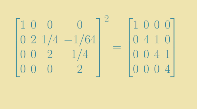
- Jordan Canonical Form: For a general matrix \( A \), one can use the Jordan canonical form to find its square roots. This involves expressing \( A \) as \( A = PJP^{-1} \), where \( J \) is a Jordan block matrix and \( P \) is an invertible matrix. The square root of \( A \) can then be found by taking the square root of each Jordan block.
- Schur Decomposition: Another method involves the Schur decomposition, where \( A \) is decomposed as \( A = UTU^* \), with \( U \) being a unitary matrix and \( T \) an upper triangular matrix. The square root of \( A \) can be computed from the square root of \( T \).
To illustrate, consider a \( 2 \times 2 \) matrix \( A \):
| A = | \[ \begin{pmatrix} a & b \\ c & d \\ \end{pmatrix} \] |
The square roots of \( A \) can be found by solving the equation \( B^2 = A \). If \( A \) has distinct eigenvalues, its square roots can be expressed using its eigenvectors and eigenvalues.
Methods for Computing Square Root of a Matrix
Computing the square root of a matrix is a fundamental problem in linear algebra with various methods available. Here, we detail some of the most common and effective techniques:
- Cholesky Decomposition: This method is primarily used for symmetric, positive definite matrices. The matrix \(A\) is decomposed as \(A = R^T R\), where \(R\) is an upper triangular matrix. The matrix square root \(S\) can then be approximated by \(R\).
- Eigenvalue Decomposition: For any symmetric matrix \(A\), it can be decomposed as \(A = Q \Lambda Q^T\), where \(Q\) is an orthogonal matrix, and \(\Lambda\) is a diagonal matrix with eigenvalues of \(A\). The square root of \(A\) can be found by taking the square root of each eigenvalue in \(\Lambda\) to form \(\Lambda^{1/2}\), resulting in \(A^{1/2} = Q \Lambda^{1/2} Q^T\).
- Denman-Beavers Iteration: This iterative method finds the square root by successively approximating it. Starting with initial guesses \(Y_0 = A\) and \(Z_0 = I\) (the identity matrix), the iterations proceed as follows:
- \(Y_{k+1} = \frac{1}{2} (Y_k + Z_k^{-1})\)
- \(Z_{k+1} = \frac{1}{2} (Z_k + Y_k^{-1})\)
- Newton-Schulz Iteration: Another iterative method, starting with an initial guess \(X_0\). The iterations are given by:
- \(X_{k+1} = \frac{1}{2} (X_k + X_k^{-1} A)\)
- Matrix Sign Function: For a matrix \(A\), the matrix sign function can be used to compute the square root. This involves an iterative process to find \(A^{1/2}\) using the sign function of \(A\).
Each method has its advantages and computational complexities. The choice of method depends on the properties of the matrix \(A\) and the specific requirements of the problem at hand.
Properties of Matrix Square Roots
The square root of a matrix is a matrix \( B \) such that \( B^2 = A \), where \( A \) is the original matrix. The properties of matrix square roots are intricate and can vary depending on the type of matrix and the method used to find the square root.
1. Existence
A matrix square root does not always exist. For a matrix \( A \) to have a square root, it must be possible to find another matrix \( B \) such that \( B \times B = A \). Here are some conditions and properties related to the existence of matrix square roots:
- **Positive Semi-Definite Matrices**: Every positive semi-definite matrix \( A \) has at least one square root. If \( A \) is positive definite, it has a unique positive semi-definite square root.
- **Non-Singular Matrices**: A non-singular matrix \( A \) has at least one square root. The number of distinct square roots can be determined by its Jordan canonical form.
- **General Matrices**: For a general matrix, the existence of a square root depends on its eigenvalues. Specifically, a square root exists if and only if every eigenvalue of \( A \) has a non-negative real part.
2. Uniqueness
The uniqueness of the matrix square root is not always guaranteed. The uniqueness of the square root depends on the properties of the matrix \( A \):
- **Positive Definite Matrices**: For a positive definite matrix \( A \), there is a unique positive definite matrix \( B \) such that \( B^2 = A \). This unique matrix is called the principal square root.
- **Diagonalizable Matrices**: If \( A \) is diagonalizable and its eigenvalues are non-negative, there can be multiple square roots. The square root is unique if and only if all the eigenvalues are positive and distinct.
- **Jordan Form**: If \( A \) can be put into Jordan canonical form, the number of distinct square roots can be derived from the multiplicities of the Jordan blocks and the eigenvalues.
3. Multiple Square Roots
When a matrix \( A \) has multiple square roots, their characteristics depend on the structure of \( A \) and its eigenvalues. Multiple square roots often arise in the following scenarios:
- **Complex Matrices**: Complex matrices can have multiple square roots, particularly when the matrix is not positive definite or has complex eigenvalues.
- **Non-Diagonalizable Matrices**: For matrices that are not diagonalizable, the number and form of their square roots can be more complex, often involving Jordan blocks and complex computations.
- **Symmetric Matrices**: Symmetric matrices can have symmetric square roots. However, the number of symmetric square roots depends on the specific structure and eigenvalues of the matrix.
4. Commutative Property
In general, matrix multiplication is not commutative, and this applies to matrix square roots as well. However, some special cases exhibit commutative properties:
- **Diagonal Matrices**: The square root of a diagonal matrix is also diagonal, and the square roots commute with the original matrix \( A \).
- **Normal Matrices**: If \( A \) is a normal matrix (i.e., \( AA^* = A^*A \)), the square roots are often normal, and the square root operation may commute under specific conditions.
5. Relationship to Eigenvalues
The eigenvalues of the square root \( B \) of a matrix \( A \) are related to the eigenvalues of \( A \):
- **Positive Eigenvalues**: If \( A \) has positive eigenvalues \( \lambda_i \), the eigenvalues of \( B \) will be the square roots of \( \lambda_i \), denoted \( \sqrt{\lambda_i} \).
- **Complex Eigenvalues**: If \( A \) has complex eigenvalues, the eigenvalues of \( B \) will be the principal square roots of those complex numbers, preserving the argument within a specific range.
- **Zero Eigenvalues**: If \( A \) has zero eigenvalues, the square root \( B \) will have corresponding zero eigenvalues.
6. Symmetric Square Roots
For symmetric and positive definite matrices, the square root can also be symmetric:
- **Principal Square Root**: The principal square root of a symmetric positive definite matrix is also symmetric and positive definite.
- **Symmetry Preservation**: If \( A \) is symmetric, and if \( B \) is a square root of \( A \), \( B \) may also be symmetric under specific conditions.
7. Numerical Stability
When computing the square root of a matrix, numerical stability is a crucial factor, especially for large matrices or those close to singularity:
- **Stability of Algorithms**: Different algorithms for computing matrix square roots have varying degrees of numerical stability. Iterative methods like the Denman-Beavers iteration can be more stable for specific matrix types.
- **Condition Number**: The condition number of the matrix can affect the stability of its square root. Highly conditioned matrices may result in numerically unstable square roots.
Existence and Uniqueness
The existence and uniqueness of the square root of a matrix depend on several key factors in linear algebra. Here’s a comprehensive overview:
- Conditions for Existence: A square matrix \( A \) has a square root if and only if all its eigenvalues are non-negative. This condition ensures that \( A \) can be expressed as \( A = Q \Lambda Q^{-1} \), where \( Q \) is the matrix of eigenvectors and \( \Lambda \) is a diagonal matrix of eigenvalues, each non-negative.
- Uniqueness of the Square Root: If \( A \) has a square root, it is not necessarily unique. However, if \( A \) is positive definite (all eigenvalues are positive), then its square root is unique and positive definite as well.
- Multiple Square Roots: Even when \( A \) is positive definite, there can still exist multiple square roots. These roots differ by multiplication with matrices like \( Q \) and \( Q^{-1} \), reflecting different choices of eigenvectors.
Applications of Matrix Square Roots
Matrix square roots find diverse applications across various fields due to their ability to simplify computations and solve complex problems. Here are some key applications:
- Engineering: In structural engineering, matrix square roots are used for analyzing dynamic systems, such as vibration analysis and control, where matrices represent physical properties like mass and stiffness.
- Physics: Quantum mechanics relies heavily on matrix operations, including matrix square roots, for calculations involving quantum states, evolution of systems, and probabilistic interpretations.
- Computer Science: Matrix square roots are fundamental in computer graphics for transformations, such as scaling and rotation, as well as in optimization algorithms and machine learning techniques, such as Principal Component Analysis (PCA).
Special Cases and Examples
- Diagonal Matrices
- 2x2 Matrices
- Higher-Dimensional Matrices
A diagonal matrix where each element off the main diagonal is zero can have its square root computed simply by taking the square root of each diagonal element.
For 2x2 matrices, a formula exists involving eigenvalues and eigenvectors, providing a straightforward method to compute the square root.
Higher-dimensional matrices often require more complex methods such as matrix decompositions like Cholesky or iterative methods like Denman-Beavers iteration for computing their square roots.
Common Algorithms and Implementations
The computation of the square root of a matrix is a significant problem in numerical linear algebra. Several algorithms and methods have been developed to efficiently compute matrix square roots, each with their own advantages and applications. Below are some of the most common algorithms and their implementations:
- Cholesky Decomposition
For a positive definite matrix \(A\), the Cholesky decomposition can be used to find its square root. The matrix \(A\) is decomposed into \(LL^T\), where \(L\) is a lower triangular matrix. The square root of \(A\) is then given by \(L\).
Steps:
- Decompose \(A\) into \(LL^T\).
- The matrix \(L\) is the square root of \(A\).
- Denman-Beavers Iteration
The Denman-Beavers iteration is an iterative method to compute the square root of a matrix. It involves the following iterative steps:
Steps:
- Initialize \(Y_0 = A\) and \(Z_0 = I\) (identity matrix).
- Iterate: \(Y_{k+1} = \frac{1}{2}(Y_k + Z_k^{-1})\) and \(Z_{k+1} = \frac{1}{2}(Z_k + Y_k^{-1})\) until convergence.
- Upon convergence, \(Y_k\) will be the square root of \(A\).
- Schur Decomposition
The Schur decomposition reduces a matrix to upper triangular form, after which the square root of the triangular matrix can be computed directly. The steps are as follows:
Steps:
- Compute the Schur decomposition of \(A\): \(A = Q T Q^*\), where \(Q\) is a unitary matrix and \(T\) is an upper triangular matrix.
- Compute the square root of \(T\) (denoted as \(T^{1/2}\)) using an appropriate method for triangular matrices.
- The square root of \(A\) is given by \(Q T^{1/2} Q^*\).
- Blocked Schur Algorithms
For large matrices, blocked Schur algorithms can be used to improve efficiency. These algorithms utilize blocking techniques to enhance performance and numerical stability, especially in parallel computing environments.
Steps:
- Reduce the matrix to block triangular form using Schur decomposition.
- Apply recursive or standard blocking techniques to compute the square root of the triangular blocks.
- Combine the results to form the square root of the original matrix.
- MATLAB and SciPy Implementations
Software packages like MATLAB and SciPy provide built-in functions for computing matrix square roots. These implementations typically use a combination of the aforementioned methods to ensure accuracy and efficiency.
Examples:
- In MATLAB, use
sqrtm(A)to compute the square root of a matrix \(A\). - In SciPy (Python), use
scipy.linalg.sqrtm(A)for the same purpose.
- In MATLAB, use

Challenges and Considerations
When computing the square root of a matrix, several challenges and considerations must be addressed to ensure accurate and efficient results. These challenges include numerical stability, complexity, performance, and ensuring the properties of the resultant matrix.
Numerical Stability
Numerical stability is a crucial consideration when computing matrix square roots, as small perturbations in the input matrix can lead to significant errors in the output. Ensuring stability involves selecting algorithms that minimize the propagation of rounding errors. For example, the Schur decomposition method and the Denman-Beavers iteration are known for their stability but may have different performance characteristics depending on the matrix properties.
Complexity and Performance
The computational complexity of algorithms for finding matrix square roots varies significantly. Iterative methods, such as the Denman-Beavers iteration, often require multiple iterations to converge, which can be computationally intensive. On the other hand, direct methods like Schur decomposition, although efficient for certain types of matrices, can become complex for large matrices.
Conditioning of the Matrix
The conditioning of the matrix plays a significant role in the computation of its square root. Poorly conditioned matrices can lead to inaccurate results. The condition number of a matrix indicates how much the output value can change for a small change in the input value. Algorithms need to handle such matrices carefully to avoid significant errors.
Existence of the Square Root
Not all matrices have square roots. For a matrix to have a real square root, it must be positive semidefinite. If the matrix has negative or complex eigenvalues, a real square root does not exist. In such cases, complex or generalized matrix square roots must be considered.
Uniqueness of the Square Root
While a positive definite matrix has a unique positive definite square root, other matrices can have multiple square roots. For example, a matrix with distinct eigenvalues can have up to \(2^n\) different square roots, where \(n\) is the size of the matrix. Determining the appropriate square root depends on the context and application.
Special Cases
Special cases such as diagonal and triangular matrices allow for more straightforward computation of square roots. Diagonal matrices, for example, have square roots that are also diagonal, where each element is the square root of the corresponding element in the original matrix. For triangular matrices, specialized iterative algorithms can be applied to find the square root efficiently.
Algorithm Choice
The choice of algorithm depends on the matrix's properties and the application's requirements. For instance, the Cholesky decomposition is efficient for positive definite matrices, while the Denman-Beavers iteration is more general but may require careful convergence checks. The Schur method, on the other hand, is robust and can handle a broader class of matrices, though it may be computationally expensive for large matrices.
Software Implementations
Various software packages provide implementations for computing matrix square roots, such as MATLAB's sqrtm function and SciPy's scipy.linalg.sqrtm. These implementations are optimized for different types of matrices and include built-in checks for numerical stability and conditioning.
Overall, understanding these challenges and considerations is essential for selecting the appropriate method and ensuring accurate and efficient computation of matrix square roots in practical applications.
Advanced Topics
-
Generalizations to Non-Square Matrices
While the square root of a matrix is typically discussed in the context of square matrices, the concept can be extended to non-square matrices through the use of singular value decomposition (SVD). For a given \( m \times n \) matrix \( A \), SVD allows us to express \( A \) as \( U\Sigma V^* \), where \( U \) and \( V \) are orthogonal matrices and \( \Sigma \) is a diagonal matrix containing the singular values of \( A \). The "square root" of \( A \) in this context is not a matrix \( B \) such that \( B^2 = A \), but rather a matrix that can transform \( A \) in a similar fashion. -
Matrix Pth Roots
The concept of the square root of a matrix can be extended to the pth root of a matrix, where we seek a matrix \( B \) such that \( B^p = A \). Similar to the square root, the pth root may not always exist, and when it does, it may not be unique. The computation of pth roots involves diagonalization or Jordan canonical forms for easier cases, and numerical methods for more complex matrices.
For instance, if \( A \) is diagonalizable, \( A = VDV^{-1} \) where \( D \) is a diagonal matrix, then \( A^{1/p} \) can be computed as \( V D^{1/p} V^{-1} \), where \( D^{1/p} \) is obtained by taking the pth root of each entry on the diagonal of \( D \). -
Matrix Exponentiation
Matrix exponentiation is a related advanced topic that involves raising a matrix to a power. This is particularly useful in solving systems of differential equations, among other applications. The matrix exponential \( e^A \) is defined through its Taylor series:
\[
e^A = \sum_{k=0}^{\infty} \frac{A^k}{k!}
\]
The exponential of a matrix is significant in various fields, including quantum mechanics and control theory. Computational methods for matrix exponentiation often involve Padé approximations or scaling and squaring techniques for efficiency and numerical stability.
Video giải thích về căn bậc hai của ma trận, các phương pháp tính toán và ứng dụng thực tế. Tìm hiểu cách tính căn bậc hai của ma trận một cách chi tiết và rõ ràng.
Căn Bậc Hai Của Ma Trận: Hướng Dẫn Toàn Diện
READ MORE:
Video giải thích về căn bậc hai của ma trận trong đại số tuyến tính. Tìm hiểu các phương pháp tính toán và ứng dụng thực tế của căn bậc hai của ma trận.
Căn Bậc Hai Của Ma Trận | Đại Số Tuyến Tính