Topic 3 square root x graph: Discover the intriguing world of the 3 square root x graph. This guide will help you understand and plot the function, revealing its characteristics, domain, range, and applications. Perfect for students and math enthusiasts, learn how to master this essential mathematical concept with ease and confidence.
Table of Content
- Graph of \( y = 3 \sqrt{x} \)
- Introduction to the Graph of y = 3√x
- Understanding the Square Root Function
- Transformation and Scaling of the Square Root Function
- Domain and Range of y = 3√x
- Intercepts of the Function
- Graph Characteristics and Behavior
- Step-by-Step Graph Plotting
- Key Points and Values
- Comparative Analysis with y = √x
- Applications of the Function in Real Life
- Common Mistakes and Misconceptions
- Practice Problems and Solutions
- Graphing Tools and Resources
- Summary and Conclusion
- YOUTUBE: Hướng dẫn chi tiết cách vẽ đồ thị hàm số căn bậc hai bằng cách sử dụng các phép biến đổi và vẽ điểm để minh họa. Phù hợp cho người học toán trung học và đại học.
Graph of \( y = 3 \sqrt{x} \)
The function \( y = 3 \sqrt{x} \) represents a transformation of the basic square root function \( y = \sqrt{x} \). Below is a detailed description of the characteristics and the graph of this function.
Function Definition
The function is defined as:
\[ y = 3 \sqrt{x} \]
Domain and Range
- Domain: The set of all non-negative real numbers, \( x \geq 0 \).
- Range: The set of all non-negative real numbers, \( y \geq 0 \).
Intercepts
- x-intercept: The graph intersects the x-axis at \( (0, 0) \).
- y-intercept: The graph intersects the y-axis at \( (0, 0) \).
Graph Characteristics
- The graph passes through the origin (0,0).
- As \( x \) increases, \( y \) increases. The graph becomes steeper compared to \( y = \sqrt{x} \) due to the factor of 3.
- The graph is a smooth curve in the first quadrant of the Cartesian plane.
Plot Points
To understand the shape of the graph, we can calculate and plot a few points:
| x | y |
|---|---|
| 0 | 0 |
| 1 | 3 |
| 4 | 6 |
| 9 | 9 |
| 16 | 12 |
Graph Representation
The graph of \( y = 3 \sqrt{x} \) can be visualized as follows:


READ MORE:
Introduction to the Graph of y = 3√x
The graph of \( y = 3 \sqrt{x} \) is a transformation of the basic square root function, scaled by a factor of 3. This function represents the relationship between \( x \) and \( y \) where \( y \) is three times the square root of \( x \). Understanding this graph is essential for grasping more complex mathematical concepts.
Let's explore the properties and characteristics of this graph:
- Basic Form: The basic form of the function is \( y = \sqrt{x} \). By multiplying by 3, we stretch the graph vertically.
- Domain: The set of all non-negative real numbers (\( x \geq 0 \)).
- Range: The set of all non-negative real numbers (\( y \geq 0 \)).
- Intercepts: The graph intersects the origin at (0,0).
To visualize this, we plot several points:
| x | y = 3√x |
|---|---|
| 0 | 0 |
| 1 | 3 |
| 4 | 6 |
| 9 | 9 |
| 16 | 12 |
These points help in drawing the curve more accurately. The graph starts at the origin and increases slowly at first, then more rapidly as \( x \) increases.
In summary, the graph of \( y = 3 \sqrt{x} \) is an essential function to understand due to its wide range of applications in different fields of study, including physics, engineering, and economics. By mastering this function, you will be well-prepared for more advanced mathematical concepts.
Understanding the Square Root Function
The square root function is a fundamental mathematical concept, represented by \( y = \sqrt{x} \). This function describes a relationship where \( y \) is the square root of \( x \). To fully understand the square root function, let's explore its properties, behavior, and graphical representation in detail.
Here are the key properties of the square root function:
- Domain: The domain of \( y = \sqrt{x} \) is all non-negative real numbers (\( x \geq 0 \)). This is because the square root of a negative number is not defined within the realm of real numbers.
- Range: The range of \( y = \sqrt{x} \) is all non-negative real numbers (\( y \geq 0 \)). The output of the square root function is always non-negative.
- Intercepts: The graph intersects the origin at (0,0). There are no other x-intercepts or y-intercepts.
- Increasing Function: The square root function is an increasing function, meaning that as \( x \) increases, \( y \) also increases.
To visualize the square root function, we plot several key points:
| x | y = √x |
|---|---|
| 0 | 0 |
| 1 | 1 |
| 4 | 2 |
| 9 | 3 |
| 16 | 4 |
These points help us draw the graph of \( y = \sqrt{x} \). The graph starts at the origin (0,0) and curves upward, becoming less steep as \( x \) increases. This shape reflects the fact that the rate of increase of the square root function slows down as \( x \) becomes larger.
In summary, the square root function \( y = \sqrt{x} \) is crucial for various mathematical applications. Its non-negative domain and range, along with its smooth, increasing curve, make it a fundamental concept in algebra and calculus. Understanding this function provides a solid foundation for exploring more complex mathematical topics.
Transformation and Scaling of the Square Root Function
Transforming and scaling the square root function \( y = \sqrt{x} \) involves applying various operations that alter its shape and position on the graph. One such transformation is the scaling by a factor of 3, resulting in the function \( y = 3 \sqrt{x} \). This transformation stretches the graph vertically. Let's explore the details of this transformation step by step.
Vertical Scaling
Vertical scaling involves multiplying the function by a constant factor. For the function \( y = 3 \sqrt{x} \), each value of \( y \) is three times the corresponding value of the basic square root function \( y = \sqrt{x} \). This means that every point on the graph of \( y = \sqrt{x} \) is moved vertically by a factor of 3.
Comparing the Graphs
To understand the impact of this transformation, let's compare some points from the graphs of \( y = \sqrt{x} \) and \( y = 3 \sqrt{x} \):
| x | y = √x | y = 3√x |
|---|---|---|
| 0 | 0 | 0 |
| 1 | 1 | 3 |
| 4 | 2 | 6 |
| 9 | 3 | 9 |
| 16 | 4 | 12 |
As seen in the table, for each value of \( x \), the corresponding \( y \)-value in \( y = 3 \sqrt{x} \) is three times that in \( y = \sqrt{x} \). This results in a graph that is vertically stretched, making it steeper.
Graphical Representation
The graphical representation of \( y = 3 \sqrt{x} \) starts at the origin (0,0) and curves upward, similar to \( y = \sqrt{x} \) but with a steeper incline. Here's how you can plot the graph step by step:
- Start at the origin (0,0).
- Plot key points from the table, such as (1,3), (4,6), (9,9), and (16,12).
- Connect these points with a smooth curve that starts at the origin and moves upward.
This transformed graph retains the general shape of the square root function but is stretched vertically, making it grow faster as \( x \) increases.
In summary, the transformation and scaling of the square root function to \( y = 3 \sqrt{x} \) involves a vertical stretch that amplifies each \( y \)-value by a factor of 3. This fundamental transformation illustrates how functions can be manipulated to fit different contexts and applications in mathematics.
Domain and Range of y = 3√x
Understanding the domain and range of the function \( y = 3 \sqrt{x} \) is crucial for graphing and analyzing its behavior. The domain and range describe the set of possible input values (x) and output values (y) for the function, respectively.
Domain
The domain of a function is the set of all possible values of x for which the function is defined. For \( y = 3 \sqrt{x} \), the square root operation imposes a restriction on the domain:
- Since you cannot take the square root of a negative number within the real number system, \( x \) must be greater than or equal to 0.
Therefore, the domain of \( y = 3 \sqrt{x} \) is:
\[ \text{Domain: } x \geq 0 \]
Range
The range of a function is the set of all possible values of y that the function can produce. For \( y = 3 \sqrt{x} \):
- The output of the square root function, \( \sqrt{x} \), is always non-negative because square roots of non-negative numbers are non-negative.
- Multiplying the non-negative values of \( \sqrt{x} \) by 3 will also produce non-negative values.
As \( x \) increases from 0 to infinity, \( y = 3 \sqrt{x} \) will also increase from 0 to infinity.
Therefore, the range of \( y = 3 \sqrt{x} \) is:
\[ \text{Range: } y \geq 0 \]
Graphical Representation
To further understand the domain and range, let's look at the graphical representation:
| x | y = 3√x |
|---|---|
| 0 | 0 |
| 1 | 3 |
| 4 | 6 |
| 9 | 9 |
| 16 | 12 |
The table illustrates that as \( x \) increases, \( y \) also increases, reinforcing the non-negative nature of both the domain and range.
In summary, the domain of \( y = 3 \sqrt{x} \) includes all non-negative real numbers (\( x \geq 0 \)), and the range includes all non-negative real numbers (\( y \geq 0 \)). This understanding is fundamental for accurately graphing the function and applying it in various mathematical contexts.
Intercepts of the Function
The intercepts of a function are the points where the graph crosses the x-axis and y-axis. For the function \( y = 3 \sqrt{x} \), finding these intercepts is straightforward and helps in understanding the graph's behavior.
X-Intercept
The x-intercept is the point where the graph crosses the x-axis. At this point, \( y = 0 \). To find the x-intercept, set \( y \) to 0 and solve for \( x \):
\[ 0 = 3 \sqrt{x} \]
Solving for \( x \):
\[ \sqrt{x} = 0 \]
\[ x = 0 \]
Thus, the x-intercept is:
\[ (0, 0) \]
Y-Intercept
The y-intercept is the point where the graph crosses the y-axis. At this point, \( x = 0 \). To find the y-intercept, set \( x \) to 0 and solve for \( y \):
\[ y = 3 \sqrt{0} \]
\[ y = 0 \]
Thus, the y-intercept is:
\[ (0, 0) \]
Graphical Representation
Both intercepts occur at the origin. This makes (0,0) a crucial point for the graph of \( y = 3 \sqrt{x} \). Here's a summary in a table format:
| Type | Value |
|---|---|
| X-Intercept | (0, 0) |
| Y-Intercept | (0, 0) |
In summary, the function \( y = 3 \sqrt{x} \) has both its x-intercept and y-intercept at the origin (0,0). This single point of intersection is critical in plotting and understanding the overall shape and position of the graph.
Graph Characteristics and Behavior
The graph of the function \( y = 3\sqrt{x} \) exhibits several important characteristics and behaviors. This section will explore these features in detail, providing a comprehensive understanding of the function's graphical representation.
- Shape: The graph of \( y = 3\sqrt{x} \) is a curve that starts from the origin and rises to the right, forming a smooth, increasing curve. Unlike a linear function, this graph curves upwards, reflecting the square root nature of the function.
- Domain: The domain of \( y = 3\sqrt{x} \) is \( x \geq 0 \). This is because the square root function is only defined for non-negative values of \( x \). Therefore, the graph exists only in the first quadrant of the Cartesian plane.
- Range: The range of the function is \( y \geq 0 \). As \( x \) increases, \( y \) also increases without bound, starting from 0 and extending to positive infinity.
- Intercepts: The graph of \( y = 3\sqrt{x} \) has one intercept:
- Y-intercept: At \( x = 0 \), \( y = 3\sqrt{0} = 0 \). Thus, the y-intercept is at the origin (0,0).
- Behavior as \( x \to \infty \): As \( x \) approaches infinity, \( y = 3\sqrt{x} \) also approaches infinity. The graph continues to rise gradually but never levels off, reflecting the continuous growth of the square root function.
- Behavior near the origin: As \( x \) approaches 0, \( y = 3\sqrt{x} \) approaches 0. Near the origin, the graph starts very flat and then begins to rise more steeply.
- Symmetry: The graph of \( y = 3\sqrt{x} \) is not symmetric. It is defined only for non-negative \( x \)-values and thus only appears in the first quadrant.
- Concavity: The graph of \( y = 3\sqrt{x} \) is concave down. This is because the second derivative of \( y = 3\sqrt{x} \) is negative, indicating that the slope of the graph decreases as \( x \) increases.
- Asymptotes: The graph of \( y = 3\sqrt{x} \) does not have any vertical or horizontal asymptotes. It continues to rise indefinitely as \( x \) increases.
Overall, the graph of \( y = 3\sqrt{x} \) displays a clear, predictable pattern, starting from the origin and rising to the right. Its characteristics make it a fundamental example of a square root function scaled by a factor of 3, providing insights into its behavior through its domain, range, intercepts, and concavity.
Step-by-Step Graph Plotting
To plot the graph of \( y = 3\sqrt{x} \), follow these detailed steps:
- Understand the function:
The function \( y = 3\sqrt{x} \) involves the square root of \( x \) scaled by a factor of 3. This means that for every value of \( x \), the corresponding \( y \) value will be three times the square root of \( x \).
- Determine the domain and range:
- Domain: Since the square root function is only defined for non-negative values, the domain of \( y = 3\sqrt{x} \) is \( x \geq 0 \).
- Range: The range is \( y \geq 0 \) as the output will also be non-negative.
- Create a table of values:
Choose a set of \( x \) values and compute the corresponding \( y \) values. Here are some examples:
\( x \) \( y = 3\sqrt{x} \) 0 \( 3\sqrt{0} = 0 \) 1 \( 3\sqrt{1} = 3 \) 4 \( 3\sqrt{4} = 6 \) 9 \( 3\sqrt{9} = 9 \) 16 \( 3\sqrt{16} = 12 \) - Plot the points on a graph:
Use the values from your table to plot points on the Cartesian plane. For example, plot (0, 0), (1, 3), (4, 6), (9, 9), and (16, 12).
- Draw the curve:
Connect the plotted points with a smooth curve. The graph should start at the origin (0, 0) and rise to the right, gradually increasing.
- Check the graph:
Ensure that the graph matches the characteristics of \( y = 3\sqrt{x} \), rising smoothly without any breaks, and that it lies entirely in the first quadrant.
- Use graphing tools:
For a more precise graph, use online graphing tools such as or . These tools allow you to input the function and visualize the graph accurately.
By following these steps, you can accurately plot the graph of \( y = 3\sqrt{x} \) and understand its behavior.
Key Points and Values
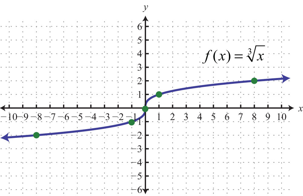
The function \( y = \sqrt[3]{x} \) has distinct characteristics that are important for understanding its graph and behavior. Below are some key points and values that help in analyzing and plotting the graph effectively.
- Domain: The domain of \( y = \sqrt[3]{x} \) is all real numbers (\( -\infty, \infty \)). This is because the cube root function is defined for all real values of \( x \).
- Range: The range is also all real numbers (\( -\infty, \infty \)), as the output of the cube root function can be any real number.
- Intercepts:
- x-intercept: The graph intersects the x-axis at \( (0,0) \).
- y-intercept: The graph intersects the y-axis at \( (0,0) \).
- Symmetry: The function \( y = \sqrt[3]{x} \) is symmetric about the origin, indicating that it is an odd function. This can be seen because \( \sqrt[3]{-x} = -\sqrt[3]{x} \).
- Behavior:
- As \( x \) approaches \( \infty \), \( y \) also approaches \( \infty \).
- As \( x \) approaches \( -\infty \), \( y \) approaches \( -\infty \).
Here are some specific points that are often useful when graphing the function:
| x | y |
|---|---|
| -8 | -2 |
| -1 | -1 |
| 0 | 0 |
| 1 | 1 |
| 8 | 2 |
These values illustrate the typical shape and growth rate of the cube root function. The function increases slowly for large values of \( x \) and \( y \), and similarly, it decreases slowly for large negative values of \( x \) and \( y \).
Understanding these key points and values will help in accurately plotting and interpreting the graph of \( y = \sqrt[3]{x} \).
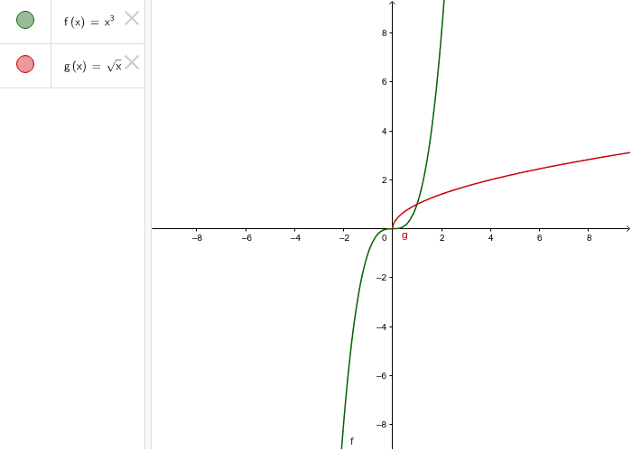
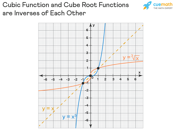
Comparative Analysis with y = √x
The graphs of \(y = \sqrt[3]{x}\) and \(y = \sqrt{x}\) share similarities but also exhibit key differences due to the nature of their respective root functions. Here, we compare these two functions in various aspects:
Graph Shape and Symmetry
- The graph of \(y = \sqrt{x}\) starts at the origin (0,0) and increases gradually, forming the right half of a parabola. It is defined only for non-negative values of \(x\) and has reflective symmetry about the line \(y = x\).
- The graph of \(y = \sqrt[3]{x}\), on the other hand, extends into both the positive and negative \(x\)-values. It passes through the origin and is symmetric about the origin (point symmetry), forming an S-shaped curve that is less steep than \(y = \sqrt{x}\).
Domain and Range
- For \(y = \sqrt{x}\):
- Domain: \(x \geq 0\)
- Range: \(y \geq 0\)
- For \(y = \sqrt[3]{x}\):
- Domain: \(x \in \mathbb{R}\) (all real numbers)
- Range: \(y \in \mathbb{R}\) (all real numbers)
Intercepts
- Both functions pass through the origin (0,0), which is their only intercept.
Behavior and Characteristics
- Increasing Behavior:
- \(y = \sqrt{x}\) increases monotonically for \(x \geq 0\). As \(x\) increases, the rate of increase of \(y\) slows down.
- \(y = \sqrt[3]{x}\) increases for \(x > 0\) and decreases for \(x < 0\). It is an odd function, meaning \(f(-x) = -f(x)\).
- Asymptotes:
- Neither function has horizontal or vertical asymptotes.
- Critical Points:
- \(y = \sqrt{x}\) has a minimum at (0,0).
- \(y = \sqrt[3]{x}\) has no relative minima or maxima but inflects at the origin, where the curve changes concavity.
Comparative Table of Values
| x | y = √x | y = ³√x |
|---|---|---|
| -8 | Undefined | -2 |
| -1 | Undefined | -1 |
| 0 | 0 | 0 |
| 1 | 1 | 1 |
| 8 | 2.83 | 2 |
Applications
- \(y = \sqrt{x}\) is commonly used in statistics, physics, and various scientific fields to model phenomena involving area, distance, and time.
- \(y = \sqrt[3]{x}\) is often used in engineering and physics to model phenomena involving volume, pressure, and other cubic relationships.
Applications of the Function in Real Life
The function \( y = \sqrt[3]{x} \) has various practical applications in real life. Understanding these applications helps illustrate the importance and utility of this mathematical concept. Below are some significant examples:
-
Physics and Engineering
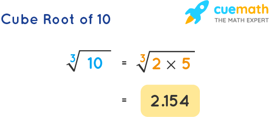
The cube root function is used in physics and engineering to model situations where the relationship between variables is non-linear. For instance, in determining the radius of a spherical object given its volume, the formula involves the cube root:
\[ r = \sqrt[3]{\frac{3V}{4\pi}} \]
-
Volume Calculations
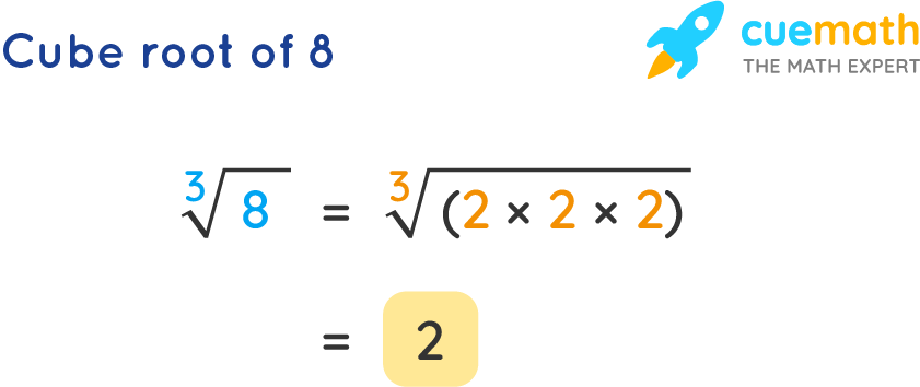
In various engineering fields, calculating the dimensions of objects based on their volume often involves the cube root. For example, the side length of a cube given its volume \( V \) is found using:
\[ s = \sqrt[3]{V} \]
-
Astronomy
In astronomy, the cube root function helps in calculating the average distance of planets from the sun, especially when using Kepler's third law, which relates the orbital period of a planet to its average distance from the sun:
\[ T^2 = k \cdot r^3 \]
where \( T \) is the orbital period, \( r \) is the average distance, and \( k \) is a constant. Solving for \( r \) involves taking the cube root:
\[ r = \sqrt[3]{\frac{T^2}{k}} \]
-
Finance
In finance, the cube root can be used to calculate the annual growth rate of investments over a multi-year period. For instance, to find the average annual growth rate \( g \) given the final value \( FV \), initial value \( IV \), and the number of years \( n \), the formula is:
\[ g = \sqrt[3]{\frac{FV}{IV}} - 1 \]
-
Biology
Biologists use the cube root function to model growth patterns in organisms, particularly when examining how volume and surface area scale with size. For example, the metabolic rate of an organism can be related to its body mass using a cube root function.
These examples illustrate how the cube root function \( y = \sqrt[3]{x} \) is applied across different fields, highlighting its versatility and importance in solving real-world problems.
Common Mistakes and Misconceptions
When studying the graph of \( y = \sqrt[3]{x} \), students often encounter several common mistakes and misconceptions. Addressing these issues is crucial for a proper understanding of the function.
-
Confusing Cube Roots with Square Roots:
A frequent error is mistaking the cube root function \( y = \sqrt[3]{x} \) for the square root function \( y = \sqrt{x} \). Unlike the square root function, which is only defined for non-negative \( x \), the cube root function is defined for all real numbers, as cube roots can be negative.
-
Ignoring Negative Inputs:
Many students incorrectly believe that the function cannot accept negative values. However, \( y = \sqrt[3]{x} \) is defined for all real \( x \), including negative numbers. For example, \( \sqrt[3]{-8} = -2 \), which means the graph extends into the third quadrant.
-
Misinterpreting the Domain and Range:
The domain and range of \( y = \sqrt[3]{x} \) are all real numbers. This is often misunderstood, leading to incomplete graphs. Correctly understanding that both the domain and range are \( (-\infty, \infty) \) is key to accurately representing the function.
-
Overlooking the Graph's Symmetry:
The graph of \( y = \sqrt[3]{x} \) is symmetric with respect to the origin. This property is essential for sketching the graph correctly, as it helps in understanding the behavior of the function in all four quadrants.
-
Incorrect Scaling:
Proper scaling is vital when plotting the graph. Incorrect scaling can distort the curve, leading to a misunderstanding of the function's nature. Ensure to use a consistent scale on both axes to accurately depict the graph.
By recognizing and correcting these common mistakes and misconceptions, students can achieve a more comprehensive understanding of the \( y = \sqrt[3]{x} \) function and its properties.
Practice Problems and Solutions
Below are a series of practice problems to help reinforce your understanding of the function \( y = 3\sqrt{x} \). Each problem is followed by a detailed solution.
-
Plot the graph of \( y = 3\sqrt{x} \) for \( x = 0, 1, 4, 9 \).
Solution:
- For \( x = 0 \): \( y = 3\sqrt{0} = 0 \) (Point: \( (0,0) \))
- For \( x = 1 \): \( y = 3\sqrt{1} = 3 \) (Point: \( (1,3) \))
- For \( x = 4 \): \( y = 3\sqrt{4} = 6 \) (Point: \( (4,6) \))
- For \( x = 9 \): \( y = 3\sqrt{9} = 9 \) (Point: \( (9,9) \))
Plot these points on the graph and draw a smooth curve through them to represent the function.
-
Determine the domain and range of \( y = 3\sqrt{x} \).
Solution:
- The domain of \( y = 3\sqrt{x} \) is \( x \geq 0 \).
- The range of \( y = 3\sqrt{x} \) is \( y \geq 0 \).
-
Find the x-intercept and y-intercept of \( y = 3\sqrt{x} \).
Solution:
- The x-intercept occurs where \( y = 0 \). Setting \( 3\sqrt{x} = 0 \) gives \( x = 0 \).
- The y-intercept occurs where \( x = 0 \). Setting \( x = 0 \) gives \( y = 0 \).
- Thus, the intercept is at \( (0,0) \).
-
Solve \( 3\sqrt{x} = 6 \) for \( x \).
Solution:
- Divide both sides by 3: \( \sqrt{x} = 2 \).
- Square both sides: \( x = 4 \).
- Thus, \( x = 4 \) is the solution.
-
Compare the graphs of \( y = \sqrt{x} \) and \( y = 3\sqrt{x} \).
Solution:
- Both graphs have the same shape, but \( y = 3\sqrt{x} \) is stretched vertically by a factor of 3.
- For example, at \( x = 1 \), \( y = \sqrt{1} = 1 \) and \( y = 3\sqrt{1} = 3 \).
- At \( x = 4 \), \( y = \sqrt{4} = 2 \) and \( y = 3\sqrt{4} = 6 \).
These practice problems should help solidify your understanding of the function \( y = 3\sqrt{x} \) and its characteristics.
Graphing Tools and Resources
When graphing the function \( y = \sqrt[3]{x} \), several online tools and resources can make the process easier and more accurate. Here are some of the most useful graphing tools and resources available:
-
Desmos Graphing Calculator:
The Desmos Graphing Calculator is a highly intuitive and versatile tool for plotting functions, including \( y = \sqrt[3]{x} \). It allows you to enter the function and instantly visualize the graph. You can interact with the graph, adjust the view, and explore key points. Desmos also provides options to add sliders, which can be useful for understanding transformations and parameter changes.
-
Mathway:
Mathway is another excellent tool for graphing and solving mathematical problems. It supports a wide range of functions and offers step-by-step solutions. For graphing \( y = \sqrt[3]{x} \), you can enter the function and see the graph along with key points and intersections. Mathway is available both as a web application and a mobile app.
-
GeoGebra:
GeoGebra is a dynamic mathematics software that brings together geometry, algebra, and calculus. It is particularly useful for visualizing and exploring mathematical concepts. GeoGebra allows you to graph \( y = \sqrt[3]{x} \) and manipulate the graph to see how changes in the function or additional parameters affect its shape.
-
Symbolab:
Symbolab provides an advanced graphing calculator that supports a wide range of functions, including radicals and polynomials. It offers detailed step-by-step solutions and interactive graphs. Enter the function \( y = \sqrt[3]{x} \) to see the graph and analyze its properties.
-
Purplemath:
Purplemath offers tutorials and resources for understanding and graphing square root functions, which can be adapted for cube root functions like \( y = \sqrt[3]{x} \). It provides detailed explanations and examples that can help you understand the principles behind graphing these functions.
These tools provide a variety of features that make it easier to graph and understand the behavior of the function \( y = \sqrt[3]{x} \). Whether you are a student, educator, or just someone interested in mathematics, these resources can help you explore and visualize mathematical concepts effectively.
Summary and Conclusion
The function \( y = \sqrt[3]{x} \) offers a unique perspective on root functions with its distinct characteristics and behavior. By examining its graph, we gain insights into its various properties such as domain, range, and symmetry.
The primary features of the graph include:
- Domain and Range: The domain and range of \( y = \sqrt[3]{x} \) are all real numbers (\( \mathbb{R} \)), indicating that the function is defined and produces real outputs for any real input.
- Intercepts: The function intersects the origin (0,0), serving as both the x-intercept and y-intercept, which is a key reference point for plotting.
- Symmetry: The graph is symmetric with respect to the origin, highlighting its odd function property (\( f(-x) = -f(x) \)).
- Behavior: As \( x \) approaches positive infinity, \( y \) increases, and as \( x \) approaches negative infinity, \( y \) decreases, illustrating the unbounded nature of the function.
In practical applications, understanding the cube root function is essential in various scientific and engineering contexts, particularly when dealing with volume calculations, scaling problems, and other scenarios where inverse operations are required.
In conclusion, mastering the graph of \( y = \sqrt[3]{x} \) provides a solid foundation for more complex mathematical explorations and real-world problem-solving. By recognizing its key points, transformations, and applications, we can effectively utilize this function in diverse fields.
Hướng dẫn chi tiết cách vẽ đồ thị hàm số căn bậc hai bằng cách sử dụng các phép biến đổi và vẽ điểm để minh họa. Phù hợp cho người học toán trung học và đại học.
Đồ Thị Hàm Số Căn Bậc Hai Bằng Cách Sử Dụng Biến Đổi & Vẽ Điểm
READ MORE:
Hướng dẫn chi tiết cách vẽ đồ thị hàm số căn bậc ba trong môn Đại Số. Phù hợp cho người học toán trung học và đại học.
Đồ Thị Hàm Số Căn Bậc Ba | Đại Số