Square Root of Minus 1: Unveiling the Mysteries of Imaginary Numbers

The concept of the square root of minus 1 is a fundamental topic in complex number theory and is represented by the imaginary unit denoted as i. This imaginary unit is essential in extending the real number system to the complex number system.

Definition

The imaginary unit i is defined by the property:

\(i = \sqrt{-1}\)

By definition, i satisfies the equation:

Properties of Imaginary Numbers

• Basic Powers of i:

  • \(i^0 = 1\)
  • \(i^1 = i\)
  • \(i^2 = -1\)
  • \(i^3 = -i\)
  • \(i^4 = 1\)

• Cyclic Nature: The powers of i repeat every four steps. This periodicity can be expressed as:

  \(i^{n+4} = i^n\)

Complex Numbers

A complex number is composed of a real part and an imaginary part and is generally expressed in the form:

\(z = a + bi\)

where:

• a is the real part.
• b is the imaginary part.

Operations with Complex Numbers

Here are some fundamental operations involving complex numbers:

Addition

The sum of two complex numbers \(z_1 = a + bi\) and \(z_2 = c + di\) is given by:

\(z_1 + z_2 = (a + c) + (b + d)i\)

Subtraction

The difference of two complex numbers \(z_1 = a + bi\) and \(z_2 = c + di\) is given by:

\(z_1 - z_2 = (a - c) + (b - d)i\)

Multiplication

The product of two complex numbers \(z_1 = a + bi\) and \(z_2 = c + di\) is given by:

\(z_1 \cdot z_2 = (ac - bd) + (ad + bc)i\)

Division

The division of two complex numbers \(z_1 = a + bi\) by \(z_2 = c + di\) is given by:

\(\frac{z_1}{z_2} = \frac{(ac + bd) + (bc - ad)i}{c^2 + d^2}\)

Applications

The imaginary unit i and complex numbers are widely used in various fields such as:

• Electrical engineering for analyzing AC circuits.
• Control theory in engineering systems.
• Quantum physics for wave functions.
• Applied mathematics for solving differential equations.

The square root of minus 1 is a concept that extends our understanding of numbers beyond the real number line. This value is represented by the imaginary unit, denoted as i, and is fundamental to complex numbers.

To comprehend the imaginary unit, consider the following:

• In real numbers, no square root exists for negative values. For instance, there is no real number that satisfies \(x^2 = -1\).
• The introduction of i allows mathematicians to define the square root of negative numbers, where:

\(i = \sqrt{-1}\)

• By definition, i satisfies the property:

\(i^2 = -1\)

This groundbreaking concept opens up a new number system called complex numbers, which include both real and imaginary parts.

A complex number is generally expressed in the form:

\(z = a + bi\)

where:

• a is the real part.
• b is the imaginary part.

Here are some key points about the imaginary unit and complex numbers:

1. Cyclic Nature of i: The powers of i exhibit a cyclic pattern:
   • \(i^0 = 1\)
   • \(i^1 = i\)
   • \(i^2 = -1\)
   • \(i^3 = -i\)
   • \(i^4 = 1\)

   This pattern repeats every four powers, which can be expressed as:

   \(i^{n+4} = i^n\)

2. Arithmetic with Complex Numbers: Operations such as addition, subtraction, multiplication, and division can be performed with complex numbers, following specific rules:
   • Addition: \((a + bi) + (c + di) = (a + c) + (b + d)i\)
   • Subtraction: \((a + bi) - (c + di) = (a - c) + (b - d)i\)
   • Multiplication: \((a + bi)(c + di) = (ac - bd) + (ad + bc)i\)
   • Division: \(\frac{a + bi}{c + di} = \frac{(ac + bd) + (bc - ad)i}{c^2 + d^2}\)
3. Applications: The imaginary unit and complex numbers are crucial in various fields such as engineering, physics, and applied mathematics. They are used to analyze electrical circuits, model wave functions, solve differential equations, and more.

The introduction of the square root of minus 1 and the development of complex numbers have significantly expanded the scope of mathematical analysis and its applications.

The imaginary unit, denoted as i, is a fundamental mathematical concept that allows the extension of the real number system to include complex numbers. It is defined by the property:

\(i = \sqrt{-1}\)

This definition implies that:

\(i^2 = -1\)

The imaginary unit i is crucial for representing and manipulating numbers that include the square root of negative values. Here are some key properties and implications of i:

Properties of the Imaginary Unit

• Basic Powers of i:
  • \(i^0 = 1\)
  • \(i^1 = i\)
  • \(i^2 = -1\)
  • \(i^3 = -i\)
  • \(i^4 = 1\)

  The powers of i repeat every four steps, demonstrating a cyclic nature:

  \(i^{n+4} = i^n\)

• Conjugates and Moduli:
  • The complex conjugate of a complex number \(z = a + bi\) is \( \overline{z} = a - bi\).
  • The modulus (or absolute value) of a complex number \(z = a + bi\) is given by \( |z| = \sqrt{a^2 + b^2} \).
• Arithmetic Operations:

  When performing arithmetic with complex numbers, specific rules apply:

  • Addition: \((a + bi) + (c + di) = (a + c) + (b + d)i\)
  • Subtraction: \((a + bi) - (c + di) = (a - c) + (b - d)i\)
  • Multiplication: \((a + bi)(c + di) = (ac - bd) + (ad + bc)i\)
  • Division: \(\frac{a + bi}{c + di} = \frac{(ac + bd) + (bc - ad)i}{c^2 + d^2}\)
• Exponentiation:

  Exponentiation involving the imaginary unit can be expressed using Euler's formula:

  \(e^{i\theta} = \cos(\theta) + i\sin(\theta)\)

Significance of the Imaginary Unit

The imaginary unit i plays a pivotal role in various areas of mathematics and science:

• In engineering, it is used to analyze alternating current (AC) circuits and signal processing.
• In physics, it is integral to quantum mechanics and the description of wave functions.
• In applied mathematics, it helps solve differential equations and model complex systems.

By incorporating the imaginary unit, mathematicians and scientists can explore and solve problems that are impossible to address using only real numbers, thus expanding the boundaries of mathematical understanding and application.

The concept of the square root of minus 1, and the subsequent development of complex numbers, has a rich and intriguing history. It emerged from the need to solve equations that had no solutions within the realm of real numbers.

Early Beginnings

The first instances of considering the square root of negative numbers appeared in the work of ancient mathematicians. However, it was often met with skepticism and regarded as an absurd notion. The journey towards acceptance began in the 16th century with the solutions to cubic equations.

The Italian Mathematicians

During the 16th century, Italian mathematicians Gerolamo Cardano, Rafael Bombelli, and others began to encounter and work with square roots of negative numbers while solving cubic equations.

• Gerolamo Cardano: In his book "Ars Magna" (1545), Cardano introduced complex numbers in the context of solving cubic equations, although he did not fully understand or accept them.
• Rafael Bombelli: Bombelli made significant strides by systematically working with these numbers in his book "Algebra" (1572), laying the foundation for the arithmetic of complex numbers.

Development in the 17th and 18th Centuries

As mathematics evolved, so did the acceptance and understanding of complex numbers:

• René Descartes: In 1637, Descartes coined the term "imaginary" for these numbers in his work "La Géométrie". While he did not fully embrace them, his acknowledgment was crucial.
• John Wallis and Isaac Newton: Both contributed to the development of complex numbers through their work on the properties of polynomials and series expansions.

Formalization in the 18th and 19th Centuries

The formal definition and widespread acceptance of complex numbers occurred in the 18th and 19th centuries:

• Leonhard Euler: Euler made substantial contributions by linking complex numbers to trigonometry through his famous formula:

  \(e^{i\theta} = \cos(\theta) + i\sin(\theta)\)

• Carl Friedrich Gauss: Gauss provided the first rigorous definition of complex numbers as pairs of real numbers, establishing the complex plane and the geometric interpretation of complex numbers.

Modern Developments

In the modern era, complex numbers and the imaginary unit i have become indispensable tools in various fields of science and engineering. They have paved the way for advancements in:

• Electrical engineering and signal processing.
• Quantum mechanics and wave theory.
• Applied mathematics and the solution of differential equations.

The historical journey of the square root of minus 1, from a controversial idea to a cornerstone of modern mathematics, highlights the importance of challenging established notions and exploring new concepts to advance our understanding of the mathematical world.

The concept of complex numbers extends the real number system ℝ to a larger system ℂ, enabling the solution of equations that do not have solutions within ℝ. A complex number is expressed in the form \(a + bi\), where \(a\) and \(b\) are real numbers, and \(i\) is the imaginary unit, defined by the property \(i^2 = -1\).

Understanding the Imaginary Unit

The imaginary unit \(i\) is a fundamental concept in complex numbers. It allows us to extend the real number line to a complex plane. The imaginary unit is defined as:
\[ i = \sqrt{-1} \]
This definition is pivotal because it implies that the square of \(i\) is -1:
\[ i^2 = -1 \]

Formation of Complex Numbers

A complex number \(z\) is written as:
\[ z = a + bi \]
where:

• \(a\) is the real part, denoted as Re(z)
• \(b\) is the imaginary part, denoted as Im(z)

Complex Plane Representation

Complex numbers can be visualized on the complex plane, where the horizontal axis represents the real part and the vertical axis represents the imaginary part. Each complex number corresponds to a unique point on this plane.

Operations with Complex Numbers

• Addition: \((a + bi) + (c + di) = (a + c) + (b + d)i\)
• Subtraction: \((a + bi) - (c + di) = (a - c) + (b - d)i\)
• Multiplication: \((a + bi)(c + di) = (ac - bd) + (ad + bc)i\)
• Division: \(\frac{a + bi}{c + di} = \frac{(a + bi)(c - di)}{c^2 + d^2}\)

Conjugates and Moduli

The complex conjugate of \(z = a + bi\) is \( \bar{z} = a - bi \). The modulus of \(z\) is given by:
\[ |z| = \sqrt{a^2 + b^2} \]
These concepts are useful in various calculations, including division and finding powers and roots of complex numbers.

Applications of Complex Numbers

Complex numbers are essential in many fields, including engineering, physics, and applied mathematics. They are used to describe oscillations, waves, and other phenomena involving sinusoidal functions. For instance, in electrical engineering, complex numbers simplify the analysis of AC circuits.

Complex numbers are an extension of the real numbers and are represented in the form \( a + bi \), where \( a \) and \( b \) are real numbers, and \( i \) is the imaginary unit with the property \( i^2 = -1 \).

A complex number can be visualized as a point or a vector in the complex plane, also known as the Argand plane, where the x-axis represents the real part and the y-axis represents the imaginary part. This plane allows us to perform operations and visualize the behavior of complex numbers geometrically.

The basic arithmetic operations for complex numbers are defined as follows:

• Addition: Given two complex numbers \( z_1 = a + bi \) and \( z_2 = c + di \), their sum is: \[ z_1 + z_2 = (a + c) + (b + d)i \]
• Subtraction: The difference between \( z_1 = a + bi \) and \( z_2 = c + di \) is: \[ z_1 - z_2 = (a - c) + (b - d)i \]
• Multiplication: The product of \( z_1 = a + bi \) and \( z_2 = c + di \) is obtained by using the distributive property: \[ z_1 \cdot z_2 = (a + bi)(c + di) = ac + adi + bci + bdi^2 = (ac - bd) + (ad + bc)i \]
• Division: To divide \( z_1 = a + bi \) by \( z_2 = c + di \), we multiply by the conjugate of the denominator: \[ \frac{z_1}{z_2} = \frac{a + bi}{c + di} \cdot \frac{c - di}{c - di} = \frac{(a + bi)(c - di)}{c^2 + d^2} = \frac{(ac + bd) + (bc - ad)i}{c^2 + d^2} \]

The modulus of a complex number \( z = a + bi \) is its distance from the origin in the complex plane and is given by:
\[
|z| = \sqrt{a^2 + b^2}
\]

The argument of a complex number, often denoted as \( \arg(z) \), is the angle \( \theta \) that the line representing the complex number makes with the positive real axis, computed as:
\[
\theta = \tan^{-1}\left(\frac{b}{a}\right)
\]

Complex numbers can also be represented in polar form as:
\[
z = r(\cos \theta + i \sin \theta)
\]
where \( r = |z| \) is the modulus and \( \theta = \arg(z) \) is the argument.

Using Euler's formula, \( e^{i\theta} = \cos \theta + i \sin \theta \), the polar form can be compactly written as:
\[
z = re^{i\theta}
\]

Understanding these representations and operations of complex numbers is fundamental for various applications in engineering, physics, and applied mathematics.

Imaginary numbers, despite their name, have numerous practical applications across various fields. Below are some key areas where imaginary numbers play a crucial role:

• Electrical Engineering: Imaginary numbers are essential in the analysis and design of electrical circuits, particularly in understanding the behavior of alternating current (AC) circuits. They are used to represent the phase and amplitude of AC signals, facilitating calculations in circuit design and signal processing.
• Signal Processing: In signal processing, imaginary numbers are used in Fourier transforms, which are mathematical techniques to analyze and manipulate signals. Fourier transforms decompose a signal into its constituent frequencies, aiding in the design of filters and the modulation and transformation of signals.
• Quantum Physics: Imaginary numbers are integral to the formulation of quantum mechanics. They help describe the behavior of particles at subatomic levels, playing a critical role in the Schrödinger equation and other fundamental quantum theories.
• Control Systems: In control theory, imaginary numbers are used to analyze and design control systems. They simplify the stability analysis of systems by allowing the representation of system behaviors in the complex plane, which aids in predicting system responses.
• Computer Graphics: Imaginary numbers are used in computer graphics for performing operations such as rotations and scaling. They enhance the realism and functionality of digital imagery by providing efficient ways to manipulate graphical objects.
• Fluid Dynamics: In fluid dynamics, imaginary numbers assist in solving complex problems related to the flow of fluids. They contribute to advancements in aerodynamics and hydrodynamics by enabling the modeling and analysis of fluid behavior under various conditions.

These applications demonstrate the utility of imaginary numbers in solving practical problems and advancing technology, making them an indispensable tool in science and engineering.

Imaginary numbers, represented as \( j \) (or \( i \) in mathematics), play a crucial role in electrical engineering, especially in the analysis of AC (alternating current) circuits.

In AC circuits, both voltage and current are sinusoidal and can be represented as complex numbers to simplify calculations. These sinusoidal functions can be expressed in terms of their magnitude and phase angle using complex numbers, where:

• The real part represents the in-phase component.
• The imaginary part represents the quadrature (90 degrees out-of-phase) component.

For example, a voltage \( V \) might be represented as:

\( V = V_0 e^{j\theta} \)

where \( V_0 \) is the amplitude and \( \theta \) is the phase angle.

This expression can be expanded using Euler's formula:

\( V = V_0 (\cos \theta + j \sin \theta) \)

Complex Impedance

Impedance in AC circuits combines resistance (real part) and reactance (imaginary part) into a single complex number. For a circuit element with impedance \( Z \), we write:

\( Z = R + jX \)

where \( R \) is the resistance and \( X \) is the reactance.

Calculating Impedance

To find the total impedance of series or parallel circuits, we use complex addition and multiplication:

• For series circuits: \( Z_{total} = Z_1 + Z_2 + ... + Z_n \)
• For parallel circuits: \( \frac{1}{Z_{total}} = \frac{1}{Z_1} + \frac{1}{Z_2} + ... + \frac{1}{Z_n} \)

Phasor Representation

Phasors are a graphical representation of the magnitude and phase angle of sinusoidal functions using complex numbers. A phasor \( V \) can be represented as:

\( V = V_m \angle \theta \)

where \( V_m \) is the magnitude and \( \theta \) is the phase angle.

AC Power Analysis

In AC circuits, power calculations often use complex numbers to account for both real power (active power) and reactive power:

• Real Power (\( P \)) = \( V_rms I_rms \cos \theta \)
• Reactive Power (\( Q \)) = \( V_rms I_rms \sin \theta \)

The apparent power (\( S \)) is a complex number given by:

\( S = P + jQ \)

Conclusion

Imaginary numbers significantly simplify the analysis of AC circuits by allowing engineers to use complex arithmetic to solve real-world problems efficiently. This approach enhances understanding and calculation of impedance, phasors, and power in electrical engineering.

Imaginary numbers play a crucial role in quantum physics, fundamentally shaping our understanding of the quantum world. The imaginary unit \(i\) is integral to the mathematical formulation of quantum mechanics, particularly in the context of wave functions and the Schrödinger equation.

One of the most significant applications of imaginary numbers in quantum physics is in the Schrödinger equation, which describes how the quantum state of a physical system changes over time. The time-dependent Schrödinger equation is expressed as:

\(i\hbar \frac{\partial \psi}{\partial t} = \hat{H} \psi\)

Here, \( \psi \) is the wave function, \( \hbar \) is the reduced Planck's constant, and \( \hat{H} \) is the Hamiltonian operator representing the total energy of the system. The presence of the imaginary unit \(i\) ensures the wave function evolves in a manner consistent with the principles of quantum mechanics.

The wave function itself, \( \psi \), is generally a complex-valued function. The probability density of finding a particle in a given state is obtained from the square of the wave function's magnitude:

\( P(x, t) = |\psi(x, t)|^2 \)

This use of complex numbers allows for the superposition of states, a fundamental concept in quantum mechanics, where a particle can exist in multiple states simultaneously until a measurement is made.

Another key aspect is the representation of quantum operators. For example, in the case of angular momentum, the operators involve imaginary components to ensure they adhere to the required commutation relations, such as:

\[ \left[ \hat{L}_x, \hat{L}_y \right] = i\hbar \hat{L}_z \]

Complex numbers also facilitate the description of quantum entanglement, a phenomenon where the quantum states of two or more particles become intertwined. This is crucial for quantum computing and information processing, where operations on qubits (quantum bits) rely on complex coefficients to represent the superposition of states.

Moreover, recent experiments and theoretical developments have underscored the necessity of complex numbers in accurately describing quantum systems. Studies have shown that real-number-only formulations of quantum mechanics fall short in explaining certain experimental results, confirming that complex numbers are essential for a complete and accurate depiction of quantum phenomena.

In summary, imaginary numbers are not just a mathematical convenience but a fundamental component of the quantum mechanical framework, enabling the accurate description and prediction of quantum behavior.

Imaginary numbers play a crucial role in control theory, particularly in the analysis and design of control systems. Their applications help ensure the stability and performance of these systems. Here are some of the key areas where imaginary numbers are essential:

• Stability Analysis: Imaginary numbers are used in determining the stability of control systems. By analyzing the location of poles in the complex plane, engineers can predict system behavior. A system is stable if all poles have negative real parts. The presence of imaginary parts in poles indicates oscillatory behavior, which is common in stable systems.
• Frequency Response: Imaginary numbers are fundamental in analyzing the frequency response of control systems. The use of the Laplace transform converts differential equations into algebraic equations in the complex plane, making it easier to study system characteristics. The imaginary axis of the complex plane represents frequency, allowing engineers to evaluate system response at various frequencies.
• Nyquist and Bode Plots: Imaginary numbers facilitate the creation of Nyquist and Bode plots, which are graphical representations used to assess the stability and performance of control systems. These plots provide insights into gain and phase margins, crucial for designing robust systems.
• Root Locus: The root locus technique involves plotting the trajectories of system poles in the complex plane as a system parameter varies. This visualization helps engineers design controllers that achieve desired performance criteria, such as damping and transient response.

Stability Analysis Example

Consider a transfer function \(H(s)\) of a control system:

$$
H(s)=

1
s^2+s+1

The poles of the system are the roots of the denominator:

$$
s^2+s+1=0

Solving this quadratic equation using the quadratic formula \(s = \frac{-b \pm \sqrt{b^2 - 4ac}}{2a}\), where \(a = 1\), \(b = 1\), and \(c = 1\), we get:

$$
s=
-1±-3
2

=

-1
2

±

3
2

i

The roots \(s = -\frac{1}{2} \pm \frac{\sqrt{3}}{2}i\) are complex, indicating that the system exhibits oscillatory behavior but remains stable as the real part is negative.

Conclusion

In summary, imaginary numbers are integral to control theory, enabling engineers to analyze, design, and optimize control systems effectively. They provide a comprehensive framework for understanding system behavior, ensuring stability, and enhancing performance.

Imaginary numbers, specifically the imaginary unit \(i\) where \(i = \sqrt{-1}\), play a crucial role in various fields of applied mathematics. Their applications extend beyond theoretical concepts to solving real-world problems. Below are some key areas where imaginary numbers are used:

• Complex Analysis: This branch of mathematics studies functions that operate on complex numbers. It is essential for evaluating integrals, solving differential equations, and modeling physical phenomena. Complex analysis leverages the imaginary unit \(i\) to extend the real-number system into the complex plane.
• Signal Processing: Imaginary numbers are vital in the field of signal processing. Fourier transforms, which decompose signals into their frequency components, use complex numbers to represent the amplitude and phase of each frequency component. This is crucial in fields like audio engineering, telecommunications, and image processing.
• Control Theory: In control systems, complex numbers help analyze the stability and behavior of dynamic systems. The poles and zeros of a system's transfer function, often complex numbers, determine its stability and response characteristics.
• Quantum Mechanics: The fundamental equations of quantum mechanics, such as the Schrödinger equation, inherently involve complex numbers. They describe the probability amplitudes of a system's state, allowing for the calculation of probabilities of different outcomes.
• Fluid Dynamics: Complex potential theory uses complex numbers to solve problems in two-dimensional fluid flow. This approach simplifies the analysis of flow patterns around objects and through various media.
• Electromagnetic Theory: Maxwell's equations, which describe the behavior of electric and magnetic fields, often involve complex numbers. They are used to solve wave equations and analyze the propagation of electromagnetic waves.
• Vibration Analysis: Complex numbers model oscillatory systems in mechanical and structural engineering. They help determine the natural frequencies and damping characteristics of structures.

The use of imaginary numbers in these areas demonstrates their power and versatility. By extending the real number system, imaginary numbers provide tools for solving a wide range of applied mathematics problems.

Complex numbers can be visualized on the complex plane, a two-dimensional plane where the x-axis represents the real part and the y-axis represents the imaginary part of a complex number.

Complex Plane

In the complex plane, any complex number \( z = a + bi \) is represented as a point \((a, b)\), where \( a \) is the real part and \( b \) is the imaginary part. This plane is essential for understanding the geometric interpretation of complex numbers.

• Real numbers lie along the x-axis.
• Imaginary numbers lie along the y-axis.

Magnitude and Angle

The magnitude (or modulus) of a complex number \( z = a + bi \) is its distance from the origin, calculated using the formula:

\[
|z| = \sqrt{a^2 + b^2}
\]

The angle (or argument) \( \theta \) is the angle formed with the positive direction of the real axis, calculated using:

\[
\theta = \tan^{-1} \left( \frac{b}{a} \right)
\]

Polar Form

Complex numbers can also be represented in polar form as:

\[
z = r (\cos \theta + i \sin \theta)
\]

where \( r \) is the magnitude and \( \theta \) is the angle. This form is particularly useful for multiplication and division of complex numbers.

Visualization of Operations

• Addition: Adding two complex numbers corresponds to vector addition in the complex plane. For \( z_1 = a + bi \) and \( z_2 = c + di \), the sum \( z_1 + z_2 = (a+c) + (b+d)i \) is found by adding their corresponding components.
• Subtraction: Subtracting two complex numbers is similar to vector subtraction. For \( z_1 = a + bi \) and \( z_2 = c + di \), the difference \( z_1 - z_2 = (a-c) + (b-d)i \) is found by subtracting their corresponding components.
• Multiplication: Multiplying two complex numbers involves multiplying their magnitudes and adding their angles. For \( z_1 = r_1 (\cos \alpha + i \sin \alpha) \) and \( z_2 = r_2 (\cos \beta + i \sin \beta) \), the product is:

  \[
  z_1 \cdot z_2 = r_1 r_2 [\cos(\alpha + \beta) + i \sin(\alpha + \beta)]
  \]

• Division: Dividing two complex numbers involves dividing their magnitudes and subtracting their angles. For \( z_1 = r_1 (\cos \alpha + i \sin \alpha) \) and \( z_2 = r_2 (\cos \beta + i \sin \beta) \), the quotient is:

  \[
  \frac{z_1}{z_2} = \frac{r_1}{r_2} [\cos(\alpha - \beta) + i \sin(\alpha - \beta)]
  \]

Graphical Representation

Plotting complex numbers and their operations on the complex plane provides a visual way to understand their interactions. For example:

• The sum of \( 1 + 2i \) and \( 3 + 4i \) is \( 4 + 6i \), plotted as a point at \((4, 6)\).
• The product of \( 1 + i \) and \( 1 - i \) is \( 1 + i^2 = 0 \), representing a point at the origin.

Advanced Visualization

Advanced visualizations include plotting functions of complex variables, such as fractals (e.g., the Mandelbrot set) which provide deeper insights into the behavior of complex functions.

Visualization techniques make complex numbers intuitive and their properties more accessible, bridging the gap between algebraic and geometric perspectives.

Euler's formula is a fundamental equation in complex analysis that establishes a deep relationship between the exponential function and trigonometric functions. It is expressed as:

\[ e^{ix} = \cos(x) + i\sin(x) \]

This formula reveals that complex exponentiation involving the imaginary unit \(i\) can be represented using sine and cosine functions. One of the most celebrated cases of Euler's formula is when \(x = \pi\), which leads to Euler's identity:

\[ e^{i\pi} + 1 = 0 \]

Euler's identity is renowned for its beauty, as it links five fundamental mathematical constants: \(e\) (the base of the natural logarithm), \(i\) (the imaginary unit), \(\pi\) (the ratio of a circle's circumference to its diameter), 1, and 0.

Understanding Euler's Formula

To understand Euler's formula, consider the following key points:

• Series Expansion: The exponential function \(e^{ix}\) can be expanded as a power series. Comparing this with the series expansions of \(\cos(x)\) and \(\sin(x)\) demonstrates their relationship:

  
  \[
  e^{ix} = 1 + ix - \frac{x^2}{2!} - \frac{ix^3}{3!} + \frac{x^4}{4!} + \cdots
  \]

  
  \[
  \cos(x) = 1 - \frac{x^2}{2!} + \frac{x^4}{4!} - \cdots
  \]

  
  \[
  \sin(x) = x - \frac{x^3}{3!} + \frac{x^5}{5!} - \cdots

• Geometric Interpretation: Euler's formula can be visualized on the complex plane, where any complex number \(z = x + iy\) can be represented as a point. The exponential form \(e^{ix}\) traces out a circle of radius 1 in the complex plane, with the angle \(x\) measured in radians from the positive real axis.

Applications of Euler's Formula

Euler's formula has wide-ranging applications in various fields of science and engineering:

• Signal Processing: In signal processing, Euler's formula is used to analyze and design filters and to represent sinusoidal signals as exponential functions.
• Quantum Mechanics: In quantum mechanics, the wave functions of particles are often expressed using complex exponentials, simplifying the analysis of quantum states and their evolution.
• Electrical Engineering: AC circuit analysis extensively uses Euler's formula to simplify the calculations of voltages and currents in complex circuits.

Proof of Euler's Formula

One way to prove Euler's formula is by using the Taylor series expansions of \(e^{ix}\), \(\cos(x)\), and \(\sin(x)\) and showing that they match term by term:

1. Start with the Taylor series expansion of \(e^{ix}\):

   
   \[
   e^{ix} = 1 + ix + \frac{(ix)^2}{2!} + \frac{(ix)^3}{3!} + \cdots
   \]

2. Separate the series into real and imaginary parts:

   
   \[
   e^{ix} = \left(1 - \frac{x^2}{2!} + \frac{x^4}{4!} - \cdots \right) + i\left(x - \frac{x^3}{3!} + \frac{x^5}{5!} - \cdots \right)
   \]

3. Recognize these as the Taylor series for \(\cos(x)\) and \(\sin(x)\):

   
   \[
   e^{ix} = \cos(x) + i\sin(x)
   \]

Euler's formula elegantly ties together exponential functions and trigonometric functions, providing profound insights into the nature of complex numbers.

The study of polynomial equations reveals the profound significance of complex numbers. By understanding the roots of these equations, one gains insight into the foundational role complex numbers play in mathematics.

Consider a polynomial equation of degree \( n \) in the form:

\[ P(x) = a_n x^n + a_{n-1} x^{n-1} + \cdots + a_1 x + a_0 = 0 \]

where \( a_i \) are coefficients. According to the Fundamental Theorem of Algebra, every non-constant polynomial equation has at least one complex root. This implies that the equation:

\[ x^2 + 1 = 0 \]

has solutions that are not real numbers. Solving for \( x \), we get:

\[ x^2 = -1 \]

which leads to:

\[ x = \pm i \]

where \( i \) is the imaginary unit, defined as the square root of -1.

Complex Conjugates

Complex roots of polynomials with real coefficients come in conjugate pairs. For instance, if \( 2 + 3i \) is a root, then \( 2 - 3i \) is also a root. This ensures the polynomial equation has real coefficients.

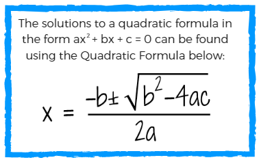
Quadratic Equations

For a quadratic equation of the form:

\[ ax^2 + bx + c = 0 \]

the roots are given by the quadratic formula:

\[ x = \frac{{-b \pm \sqrt{{b^2 - 4ac}}}}{2a} \]

If the discriminant \( b^2 - 4ac \) is negative, the roots are complex. For example, consider:

\[ x^2 + 4x + 5 = 0 \]

Here, \( a = 1 \), \( b = 4 \), and \( c = 5 \). The discriminant is:

\[ 4^2 - 4 \cdot 1 \cdot 5 = 16 - 20 = -4 \]

The roots are:

\[ x = \frac{{-4 \pm \sqrt{-4}}}{2 \cdot 1} = \frac{{-4 \pm 2i}}{2} = -2 \pm i \]

Higher-Degree Polynomials

For polynomials of degree higher than two, complex roots are found similarly. Consider the cubic equation:

\[ x^3 - 6x^2 + 11x - 6 = 0 \]

Factoring gives:

\[ (x - 1)(x - 2)(x - 3) = 0 \]

which has roots \( x = 1, 2, 3 \), all real. However, introducing complex coefficients or ensuring no real factorization necessitates complex roots. For instance:

\[ x^3 + 0x^2 + 0x + 1 = 0 \]

has one real root and two complex roots:

\[ x = -1, \quad \text{and} \quad x = \frac{1 \pm i \sqrt{3}}{2} \]

Visualization

Graphically, complex roots are often depicted on the complex plane, where the x-axis represents the real part and the y-axis represents the imaginary part of the complex number.

Visualizing complex roots helps in understanding the symmetry and distribution of roots in relation to polynomial equations.

Thus, the roots of polynomial equations deeply connect with complex numbers, showcasing their essential role in mathematics.

Imaginary numbers, particularly the imaginary unit \(i\), often give rise to various misconceptions. Here, we address some of the most common misunderstandings:

• Imaginary numbers are not "real":

  Many people think that imaginary numbers are purely fictional and have no real-world applications. In reality, imaginary numbers are a crucial part of complex numbers, which are used in many practical fields such as electrical engineering, quantum physics, and control theory.

• Imaginary numbers have no practical use:

  This is far from the truth. Imaginary numbers are used extensively in signal processing, control systems, and other engineering disciplines. For example, in electrical engineering, alternating current (AC) circuit analysis heavily relies on complex numbers.

• \(i\) is the only imaginary number:

  While \(i\), defined as \(\sqrt{-1}\), is the fundamental imaginary unit, any real number multiplied by \(i\) is also an imaginary number. Thus, numbers like \(2i\), \(-5i\), and \(\frac{3}{4}i\) are all imaginary numbers.

• Imaginary numbers cannot be visualized:

  Imaginary numbers can be represented on the complex plane, where the horizontal axis represents real numbers and the vertical axis represents imaginary numbers. This allows for a geometric interpretation of complex number operations.

• Imaginary numbers are difficult to work with:

  Although they might seem challenging at first, the arithmetic of imaginary and complex numbers follows systematic rules similar to those for real numbers. Operations such as addition, subtraction, multiplication, and division can be performed using standard algebraic methods.

Understanding these misconceptions can help demystify imaginary numbers and highlight their importance in both theoretical and applied mathematics.

Complex analysis delves into intricate concepts beyond basic operations and properties of complex numbers. Here are some advanced topics worth exploring:

1. Residue Theory: This branch deals with the calculus of residues, which are complex numbers related to the behavior of meromorphic functions around singularities. It finds extensive applications in solving integrals and evaluating complex series.
2. Conformal Mapping: Conformal mappings preserve angles locally, providing a powerful tool in various fields such as fluid dynamics, electromagnetism, and cartography. These mappings can transform complex domains into simpler shapes while preserving essential geometric properties.
3. Analytic Continuation: Analytic continuation extends the domain of validity of a complex function beyond its original definition. This technique is crucial for understanding the behavior of functions in complex plane regions where they are not initially defined and plays a pivotal role in the study of special functions and complex differential equations.
4. Riemann Surfaces: Riemann surfaces are complex manifolds that generalize the notion of a single-valued complex function. They provide a geometric framework for understanding multivalued functions, branch cuts, and the topology of complex functions.
5. Harmonic Functions: Harmonic functions are solutions to Laplace's equation and exhibit interesting properties in complex analysis. They arise in various physical and mathematical contexts, including potential theory, fluid flow, and harmonic analysis.
6. Complex Dynamics: Complex dynamics explores the behavior of iterated complex functions, particularly in the context of dynamical systems theory. This field studies the iteration of functions such as the complex exponential, logarithm, and quadratic polynomials to analyze the long-term behavior of trajectories in the complex plane.

Imaginary numbers, often misunderstood, hold profound significance across various scientific and mathematical disciplines. Here's a summary of their importance:

1. Mathematical Foundation: Imaginary numbers form the cornerstone of complex analysis, providing a rich framework for understanding functions, equations, and geometric transformations in the complex plane.
2. Physical Applications: Despite their "imaginary" label, these numbers find concrete applications in physics, particularly in quantum mechanics and electrical engineering. They represent phase shifts, oscillations, and wave functions with remarkable accuracy.
3. Control Theory: Imaginary numbers play a crucial role in control systems, aiding in the analysis and design of dynamic systems. Concepts like transfer functions and stability analysis heavily rely on complex numbers.
4. Advanced Mathematics: Imaginary numbers extend the realm of real numbers, enabling solutions to previously unsolvable equations, such as finding roots of polynomials and solving differential equations.
5. Geometric Interpretation: The geometric interpretation of complex numbers offers insights into transformations, mappings, and fractals, enriching our understanding of mathematical structures and patterns.
6. Unity of Mathematics: Imaginary numbers bridge the seemingly disparate realms of algebra and geometry, illustrating the interconnectedness of mathematical concepts and fostering interdisciplinary research.

In conclusion, the square root of minus one, though initially perplexing, reveals itself as a fundamental component of mathematical thought, unlocking new realms of understanding and application across diverse fields.